|
Lecture Notes 11 Econ
29000, Principles of Statistics Kevin R Foster, CCNY Fall
2011 |
|
|
|
Other Data: ATUS |
|
|
We will use data from the "American Time Use Survey," or ATUS. This asks respondents to carefully list how they spent each hour of their time during the day; it's a tremendous resource. The survey data is collected by the US Bureau of Labor Statistics (BLS), a US government agency. You can find more information about it here, http://www.bls.gov/tus/.
The dataset has information on 98,778 people interviewed from 2003-2009. This gives you a ton of information – we really need to work to get even the simplest information from it.
The SPSS-format data for ATUS is online, on InYourClass.com in the "Kevin SPSS" group.
The ATUS has data telling how many minutes each person spent on various activities during the day. These are created from detailed logbooks that each person kept, recording their activities throughout the day.
They recorded how much time was spent with family members, with spouse, sleeping, watching TV, doing household chores, working, commuting, going to church/religious ceremonies, volunteering – there are hundreds of specific data items!
The NY Times had this graphic showing the different uses of time during the day [here http://www.nytimes.com/interactive/2009/07/31/business/20080801-metrics-graphic.html is the full interactive chart where you can compare the time use patterns of men and women, employed and unemployed, and other groups – a great way to lose an evening! The article is here http://www.nytimes.com/2009/08/02/business/02metrics.html?_r=2 ]
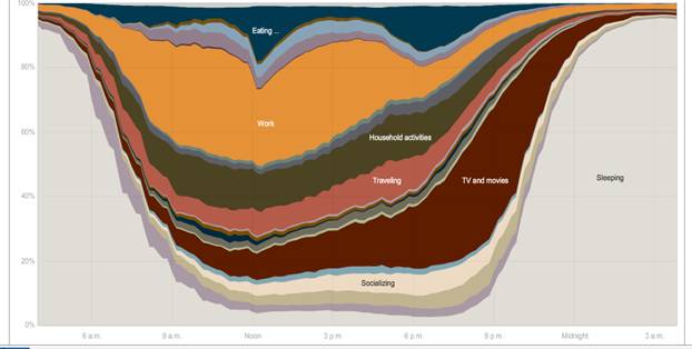
I have done some initial work on this dataset for you, classifying time into broad categories (such as seen in the graphic above). The broad categories in the graphic such as "Work" or "TV and movies" are not given in the initial data. Rather you need to add up the total time spent by people in a variety of activities.
These are coded and assembled; the summaries are provided in this file (i.e. the total number of minutes spent sleeping, but not the particular times during the day that each individual was sleeping). At the beginning are a few summary variables that I've created, including some basic coding-up into broad categories – for example, we have detailed data on time spent on aerobics, baseball, basketball, biking, ... all the way to wrestling and yoga; I added these into the category, "Time playing sports." When analyzing these, remember that in many cases the salient variation is between those with zero time spent on a particular activity and those with a non-zero time.
You might want to make your own categorizations. It is helpful to understand the ATUS classification system, where additional numbers at the right indicated additional specificity. The first two digits give generic broad categories. The general classification T05 refers to time spent doing things related to work. T0501 is specific to actual work; T050101 is "Work, main job" then T050102 is "Work, other job," T050103 is "Security Procedures related to work," and T050189 is "Working, Not Elsewhere Classified," abbreviated as n.e.c. (usually if the final digit is a nine then that means that it is a miscellaneous or catch-all category). Then there are activities that are strongly related to work, that a person might not do if they were not working at a particular job – like taking a client out to dinner or golfing. These get their own classification codes, T050201, T050202, T050203, T050204, or T050289. The list continues; there are "Income-generating hobbies, crafts, and food" and "Job interviewing" and "Job search activities." These have other classifications beginning with T05 to indicate that they are work-related.
So for instance, to create a variable, "Time Spent Working" that we might label "T_work," you would have to add up T050101, T050102, T050103, T050189, T050201, T050202, T050203, T050204, T050289, T050301, T050302, T050303, T050304, T050389, T050403, T050404, T050405, T050481, T050499, and T059999. You might want to add in "Travel related to working" down in T180501. No sane human, outside a story by Borges, would remember all these codings but you'd look at the "Labels" in SPSS and create a new variable. It's tedious but not difficult in any way. (The pdf Lexicon gives the complete list.)
You can imagine that different researchers, exploring different questions, could want different aggregates. So the basic data has a very fine classification which you can add up, however you want. I gave one classification but you can (and should) make changes.
|
Interpretation |
|
|
In many arguments, it is important show that a certain estimator is statistically significantly different from zero. But that mere fact does not "prove" the argument and you should not be fooled into believing otherwise. It is one link in a logical chain but any chain is only as strong as its weakest link. If there is strong statistical significance then this means one link of the chain is strong, but if the rest of the argument is held together by threads it will not support any weight. As a general rule, you will rarely use a word like "prove" if you want to be precise (unless you're making a mathematical proof). Instead, phrases like "consistent with the hypothesis" or "inconsistent with the hypothesis" are better, since they remind the reader of the linkage: the statistics can strengthen or weaken the argument but they are not a substitute.
A recent example: there is a correlation between student homework and exam grade; this is clearly shown in this graph:
Do you think this is causal? Does hard work tend to pay off?
Recall the use of evidence to make an argument: if you watch a crime drama on TV you'll see court cases where the prosecutor shows that the defendant does not have an alibi for the time the crime was committed. Does that mean that the defendant is guilty? Not necessarily – only that the defendant cannot be proven innocent by demonstrating that they were somewhere else at the time of the crime.
You could find statistics to show that there is a statistically significant link between the time on the clock and the time I start lecture. Does that mean that the clock causes me to start talking? (If the clock stopped, would there be no more lecture?)
There are millions of examples. In the ATUS data that I mentioned, we see that people who are not working have a statistically significant increase in time on religious activities. We find a statistically significant negative correlation between the time that people spend on religious activities and their income. Do these mean that religion causes people to be poorer? (We could go on, comparing the income of people who are unusually devout, perhaps finding the average income for quartiles or deciles of time spent on religious activity.) Of course that's a ridiculous argument and no amount of extra statistics or tests can change its essentially ridiculous nature! If someone does a hundred statistical tests of increasing sophistication to show that there is that negative correlation, it doesn't change the essential part of the argument. The conclusion is not "proved" by the statistics. The statistics are "consistent with the hypothesis" or "not inconsistent with the hypothesis" that religion makes people poor. If I wanted to argue that religion makes people wealthy, then these statistics would be inconsistent with that hypothesis.
Generally two variables, A and B, can be correlated for various reasons. Perhaps A causes B; maybe B causes A. Maybe both are caused by some other variable. Or they each cause the other (circular causality). Or perhaps they just randomly seem to be correlated. Statistics can cast doubt on the last explanation but it's tough to figure out which of the other explanations is right.
|
On Sampling |
|
|
All of these statistical results, which tell us that the sample average will converge to the true expected value, are extremely useful, but they crucially hinge on starting from a random sample -- just picking some observations where the decision on which ones to pick is done completely randomly and in a way that is not correlated with any underlying variable.
For example if I want to find out data about a typical New Yorker, I could stand on the street corner and talk with every tenth person walking by – but my results will differ, depending on whether I stand on Wall Street or Canal Street or 42nd Street or 125th Street or 180th Street! The results will differ depending on whether I'm doing this on Friday or Sunday; morning or afternoon or at lunchtime. The results will differ depending on whether I sample in August or December. Even more subtly, the results will differ depending on who is standing there asking people to stop and answer questions (if the person doing the sample is wearing a formal suit or sweatpants, if they're white or black or Hispanic or Asian, if the questionnaire is in Spanish or English, etc).
In medical testing the gold standard is "randomized double blind" where, for example, a group of people all get pills but half get a placebo capsule filled with sugar while the other half get the medicine. This is because results differ, depending on what people think they're getting; evaluations differ, depending on whether the examiner thinks the test was done or not. (One study found that people who got pills that they were told were expensive reported better results than people who got pills that were said to be cheap – even though both got placebos.)
Getting a true random sample is tough. Randomly picking telephone numbers doesn't do it since younger people are more likely to have only a mobile number not a land line and poorer households may have more people sharing a single land line. Online polls aren't random (as a general rule, never believe an online poll about anything). Online reviews of a product certainly aren't random. Government surveys such as the ones we've used are pretty good – some smart statisticians worked very hard to ensure that they're a random sample. But even these are not good at estimating, say, the fraction of undocumented immigrants in a population.
There are many cases that are even subtler. This is why most sampling will start by reporting basic demographic information and comparing this to population averages. One of the very first questions to be addressed is, "Are the reported statistics from a representative sample?"
|
On Bootstrapping |
|
|
Recall the whole rationale for our method of hypothesis testing. We know that, if some average were truly zero, it would have a normal distribution (if enough observations; otherwise a t distribution) around zero. It would have some standard error (which we try to estimate). The mean and standard error are all we need to know about a normal distribution; with this information we can answer the question: if the mean were really zero, how likely would it be, to see the observed value? If the answer is "not likely" then that suggests that the hypothesis of zero mean is incorrect; if the answer is "rather likely" then that does not reject the null hypothesis.
This depends on us knowing (somehow) that the mean has a normal distribution (or a t distribution or some known distribution). Are there other ways of knowing? We could use computing power to "bootstrap" an estimate of the significance of some estimate.
This "bootstrapping" procedure was done in a previous lecture note, on polls of the household income.
Although differences in averages are distributed normally (since the averages themselves are distributed normally, and then linear functions of normal distributions are normal), we might calculate other statistics for which we don't know the distributions. Then we can't look up the values on some reference distribution – the whole point of finding Z-statistics is to compare them to a standard normal distribution. For instance, we might find the medians, and want to know if there are "big" differences between medians.
Follow the same basic procedure: take the whole dataset, treat it as if it were the population, and sample from it. Calculate the median of each sample. Plot these; the distribution will not generally have a Normal distribution but we can still calculate bootstrapped p-values.
For example, suppose I have a sample of 100 observations with a standard error equal to 1 (makes it easy; i.e. the standard error is 10 and 10/sqrt(100) = 1) and I calculate that the average is 1.95. Is this "statistically significantly" different from zero?
One way to answer this is to use the computer to create lots and lots of samples, from a population with a zero mean and standard error of 1, and then count up how many are farther from zero than 1.95. Or we can use the Standard Normal distribution to calculate the area in both tails beyond 1.95 to be 5.12%. When I bootstrapped values I got answers pretty close (within 10 bps) for 10,000 simulations. More simulations would get more precise values.
So let's try a more complicated situation. Imagine two distributions have the same mean; what is the distribution of median differences? I get this histogram of median differences:
So clearly a value beyond about 0.15 would be pretty extreme and would convince me that the real distributions do not have the same median. So if I calculated a value of -0.17, this would have a low bootstrapped p-value.