Lecture Notes 6

Econ 29000, Principles of Statistics

Kevin R Foster, CCNY

Fall 2011

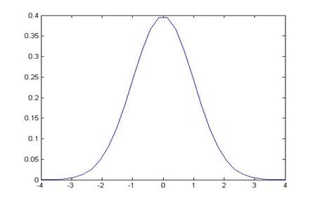
Wrap-up and Review: Calculating Area under Normal Distribution

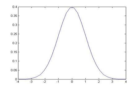
It might be useful, when thinking about Normal distributions, to consider much of the work as just a change of measurement units along the x-axis. A Standard Normal (with zero mean and standard deviation of one) can be thought of as just a change of units away from a Normal (with some non-zero mean and standard deviation other than one).

For example, the question, " For a Normal Distribution with mean 4 and standard deviation 6, what is area to the left of 1?" We can graph this as:

or it can be equivalently graphed with a change of units, by subtracting the mean (4) and dividing by the standard deviation (6):

It's the same area under either distribution – it doesn't matter whether we use the red units or the blue units; we get the same answer. The blue units are "standardized" while the red are not; for the blue units we use a standard normal distribution while for the red units we use a normal distribution with a different mean and standard deviation.

Examples of Standard Normal Calculations

Just Pictures

Find:

Given:

=0.79

Or, given

=0.29

Or, given

=0.21

Find

Given

=0.36

Or, given

=0.86

Or, given

=0.14

1. A random variable is distributed as a standard normal. Sketch the PDF in each case. Find the Z-statistics.

a. What is the probability that we could observe a value as far or farther than 1.3?

b. What is the probability that we could observe a value nearer than 1.8?

c. What value would leave 10% of the probability in the right-hand tail?

d. What value would leave 25% in both the tails (together)?

A random variable is distributed with mean of 7 and standard deviation of 9.

e. What is the probability that we could observe a value lower than 6?

f. What is the probability that we could observe a value higher than 12?

g. What is the probability that we'd observe a value between 6.5 and 7.5?

h. What is the probability that the standardized value lies between 0.5 and -0.5?

(these questions were on previous year's exams.)

a. What is the probability that we could observe a value as far or farther than 1.3? Sketch this picture:

Using Excel, we can find the area to the left of -1.3, this is NORMSDIST(-1.3):

Which is 0.0968. To find the area of both tails we just multiply by two since they're symmetric so the total area is 0.1936.

Could instead solve this by finding NORMSDIST(1.3) which is the area to the left of 1.3, so:

Which is 0.9032. So subtract this from 1 to find the remaining area in the right-hand tail, which is 0.0968.

Then multiply by two to find the area of both tails – getting the exact same answer as before.

A standard normal table might give the area of the right-hand tail.

b. What is the probability that we could observe a value nearer than 1.8?

Sketch as:

Again using Excel gives NORMSDIST(-1.8) = 0.03593, which is this area:

So multiply by 2 to find the area of both tails,

Then subtract this combined area from 1 to find the remaining middle area: 1 – 0.03593 – 0.03593 = 0.9281.

c. What value would leave 10% of the probability in the right-hand tail?

Want to find some Z such that P{X>Z} = 0.10. Use the inverse function on Excel, NORMSINV(0.10) to find that this is -1.28.

Z

But why a negative number? Again, because Excel is giving the area to the left; but the standard normal is symmetric so Z=1.28 gives the answer.

d. What value would leave 25% in both the tails (together)?

Now we want to find Z that leaves 25% in each tail; i.e. 12.5% or 0.125. Again use NORMSINV(0.125) = -1.15, so the area less than -1.15 and greater than +1.15 is 0.25.

-Z

+Z

e. What is the probability that we could observe a value lower than 6?

This is for a Normal distribution with mean 7 and standard deviation of 9, not a standard normal (mean zero and stdev 1). We need to work back-and-forth between the two distributions, finding a way to "translate" between horizontal axes.

First note how we could re-label the Standard Normal axis is the picture above, if we think of the numerals as representing standard deviations from the mean. So the mean is seven; translate zero as seven:

How do we fill in the rest? Each standard deviation has size 9, so 1 standard deviation above the mean is 7 + 9 = 16.

Then one standard deviation less than the mean is 7 – 9 = -2.

Then fill in above and below to get:

So to find the area below 6 is:

The formula for this back-and-forth was given in previous lectures. If X has a Normal Distribution with mean µ and standard deviation σ, then Z has a Standard Normal distribution with mean of 0 and standard deviation of 1, where (re-write as , which is the formula used to "translate" the horizontal axis above).

So the area above, to the left of 6 (measured in X-units) is equivalently the area to the left of . Look this up with Excel: NORMSDIST(-1/9) = 0.4558. This seems about right since we know that the area to the left of zero is 0.5; this is just a bit to the left so it's just a bit less than 50%.

f. What is the probability that we could observe a value higher than 12?

-29 -20 -11 -2 7 16 25 34 43

So translate 12 as equivalent to ; lookup in Excel as NORMSDIST(5/9) = 0.7107.

g. What is the probability that we'd observe a value between 6.5 and 7.5?

This is the little slice:

-29 -20 -11 -2 7 16 25 34 43

Between 6.5, which translates as and 7.5 which is . We can calculate NORMSDIST(-1/18) = 0.4778; this means that the area between -1/18 and zero must be 0.5 – 0.4778 = 0.0222, so the symmetric area from zero to +1/18 is the same size so the total area must be 0.0443.

h. What is the probability that the standardized value lies between 0.5 and -0.5?

This doesn't require translation since it's already translated to standardized values; 0.5 standard deviations from 7 is 7 ± 4.5 so 2.5 and 11.5. The probability to the left of- 0.5 is NORMSDIST(-0.5) = 0.3085 so the area from -0.5 to zero must be 0.5 – 0.3085 = 0.1915. Twice this area is 0.3829.