Lecture Notes 8

Econ 29000, Principles of Statistics

Kevin R Foster, CCNY

Fall 2011

About Midterm:

Midterm is on Friday october 14, 12:30-1:45pm, in location TBD. Or bring your own if you prefer the home-field advantage.

Exam is open book, open notes, open internet. The only restriction is on communications, where an answer to the specific problem posed on the exam is requested. No real-time communication of any type is allowed during the exam.

Exam answers can be put on computer or in blue books or any combination.

Exams are graded 'blind' so you only identify by your ID number.

Complications from a Series of Hypothesis Tests

Often a modeler will make a series of hypothesis tests to attempt to understand the inter-relations of a dataset. However while this is often done, it is not usually done correctly. Recall from our discussion of Type I and Type II errors that we are always at risk of making incorrect inferences about the world based on our limited data. If a test has an significance level of 5% then we will not reject a null hypothesis until there is just a 5% probability that we could be fooled into seeing a relationship where there is none. This is low but still is a 1-in-20 chance. If I do 20 hypothesis tests to find 20 variables that significantly impact some variable of interest, then it is likely that one of those variables is fooling me (I don't know which one, though). It is also likely that my high standard of proof meant that there are other variables which are more important but which didn't seem it.

Sometimes you see very stupid people who collect a large number of possible explanatory variables, run hundreds of regressions, and find the ones that give the "best-looking" test statistics – the ones that look good but are actually entirely fictitious. Many statistical programs have procedures that will help do this; help the user be as stupid as he wants.

Why is this stupid? It completely destroys the logical basis for the hypothesis tests and makes it impossible to determine whether or not the data are fooling me. In many cases this actually guarantees that, given a sufficiently rich collection of possible explanatory variables, I can run a regression and show that some variables have "good" test statistics – even though they are completely unconnected. Basically this is the infamous situation where a million monkeys randomly typing would eventually write Shakespeare's plays. A million earnest analysts, running random regressions, will eventually find a regression that looks great – where all of the proposed explanatory variables have test statistics that look great. But that's just due to persistence; it doesn't reflect anything about the larger world.

In finance, which throws out gigabytes of data, this phenomenon is common. For instance there used to be a relationship between which team won the Super Bowl (in January) and whether the stock market would have a good year. It seemed to be a solid result with decades of supporting evidence – but it was completely stupid and everybody knew it. Analysts still work to get slightly-less-implausible but still completely stupid results, which they use to sell their securities.

Consider the logical chain of making a number of hypothesis tests in order to find one supposedly-best model. When I make the first test, I have 5% chance of making a Type I error. Given the results of this test, I make the second test, again with a 5% chance of making a Type I error. The probability of not making an error on either test is (.95)(.95) = .9025 so the significance level of the overall test procedure is 1 - .9025 = 9.75%. If I make three successive hypothesis tests, the probability of not making an error is .8574 so the significance level is 14.26%. If I make 10 successive tests then the significance level is over 40%! This means that there is a 40% chance that the tester is being fooled, that there is not actually the relationship there that is hypothesized – and worse, the stupid tester believes that the significance level is just 5%.

Hypothesis Testing with two samples

In our examples we have often come up with a question where we want to know if there is a difference in mean between two groups. From the PUMS data, we could ask if, say, people in NYC are paying too much of their income to rent (where "too much" is generally defined as one-third).

For the PUMS data, SPSS tells us (using "Analyze \ Descriptive Statistics \ Descriptives") that, of 74,793 households, the average "Gross Rent as percent of income" in the sample is 40, with a standard deviation of 28.89. So the standard error of the average is = 0.1056; so two standard errors from 40 is still only 39.7887 and 40.2113; the ideal amount of 33% of income is over 66 standard errors away! We don't need to look up NORMSDIST(-66) to figure that this is highly improbable. We might want to subdivide farther: to look if the burden of rent is worse in Manhattan, say, compared with the other boroughs.

Now we find that in Manhattan the fraction of income going to rent is 37.79 with standard deviation of 27.608, against 41.62 (with standard error of 29.213) for the outer boroughs (SPSS output in appendix below). Are these significantly different from each other? Could we just be observing a difference that is within the range of variation that we'd expect, given such a diverse group of households? Are they statistically significantly different from each other? Our formula that we learned last time has only one n – what do we do if we have two samples?

Basically we want to figure out how to use the two separate standard errors to estimate the joint standard error; once we get that we'll use the same basic strategy to get our estimate, subtract off the null hypothesis (usually zero), and divide by its standard error. We just need to know what is that new standard error.

To do this we use the sum of the two sample variances: if we are testing group 1 vs group 2, then a test of just group 1 would estimate its variance as , a test of group 2 would use , and a test of the group would estimate the standard error as .

We can make either of two assumptions: either the standard deviations are the same (even though we don't know them) or they're different (even though we don't know how different). It is more conservative to assume that they're different (i.e. don't assume that they're the same) – this makes the test less likely to reject the null.

More examples

Look at the burden of rent by household type (single vs married) in the PUMS data. (Either "Analyze \ Descriptive Statistics \ Explore" or "Analyze \ Reports \ Case Summaries" then un-click "display cases," put in "Gross Rent as percent of income" as "Variable(s)" and "Household Type" into "Grouping Variable(s)" and choose from "Statistics" to get "Number of cases," "Mean," and "Standard Deviation" to get fewer extra stats.)

Gross Rent as percent of income
Household Type	N	Mean	Std. Deviation
married couple	20581	33.17	25.397
male householder no wife	3834	35.42	26.344
female householder no husband	15654	45.05	31.213
male householder living alone	11520	41.93	29.555
not living alone	3255	30.92	23.826
female householder living along	16893	46.33	29.745
other	3056	33.29	24.506
Total	74793	40.00	28.893

The first three categories are householders (usually with families) either married (20,581 households), headed by a male (only 3834) or headed by a female (15,654 households). The remainder are living alone or in other household structures so we will ignore them for now.

Married couples have a mean rent as fraction of income as 33.17. The standard error of this mean is 25.397/sqrt(20581) = 0.178. So what is the likelihood that married couples have a mean of 33 percent of income devoted to rent, but we could observe a number as high or higher as 33.17? This is just under one standard error away. Graph this normal distribution as either:

or, standardized,

So the area in the right tail is 16.98%; the probability of seeing a difference as far away as 33.17 or farther (in either direction) is 33.96%. So we cannot reject the null hypothesis that the true value is 33% but we could observe this difference.

By contrast, the average burden of rent for female-headed households is 45.05%; this average has a standard error of 31.213/sqrt(15654) = .249. So 45.05 is 12.05 away from 33, which is (45.05 – 33)/.249 = 48.3 standard errors away from the mean!

It is almost silly to graph this:

since we note that the right tail goes only as high as 34 so 45 would be far off the edge of the page, with about a zero probability.

So we can reject the null hypothesis that female-headed households devote 33% of their income to rent since there is almost no chance that, if the true value were 33%, we could observe a value as far away as 45%.

Alternately we could construct confidence intervals for these two averages: married couples pay 33.17 ± 1.96*0.178 fraction of income to rent; this is 33.17 ± .349, the interval (32.821, 33.519) which includes 33%. Female-headed households pay 45.05 ± 1.96*.245 = 45.05 ± .489, the interval (44.561, 45.539), which is far away from 33%.

Recall: why 1.96? Because the area under the normal distribution, within ±1.96 of the mean (of zero) has area of 0.95; alternately the area in the tails to the left of -1.96 and to the right of 1.96 is 0.05.

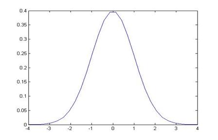
The area in blue is 5%; the area in the middle is 95%.

Alternately we could form a statistic of the difference in averages. This difference is 45.05 – 33.17 = 11.88. What is the standard error of this difference? Use the formula so it is sqrt[ (31.213)²/15654 + (25.397)²/20581 ] = sqrt( .062 + .031 ) = .306. So the difference of 11.88 is 11.88/.306 = 38.8 so nearly 39 standard errors away from zero. Again, this means that there is almost zero probability that the difference could actually be zero and yet we'd observe such a big difference.

To review, we can reject, with 95% confidence, the null hypothesis of zero if the absolute value of the z-statistic is greater than 1.96, where . Re-arrange this to state that we reject if , which is equivalent to the statement that we can reject if .

To construct a 99% confidence interval, we'd have to find the Z that brackets 99% of the area under the standard normal – you should be able to do this. Then use that number instead of 1.96. For a 90% confidence interval, use a number that brackets 90% of the area and use that number instead of 1.96.

P-values

If confidence intervals weren't confusing enough, we can also construct equivalent hypothesis tests with p-values. Where the Z-statistic tells how many standard errors away from zero is the observed difference (leaving it for us to know that more than 1.96 implies less than 5%), the p-value calculates this directly.

So to find p-values for the averages above, for fraction of income going to rent for married or female-headed households, find the probabilities under the normal for the standardized value (for married couples) of (33.17 – 33)/.178 = .955; this two-tailed probability is 33.96% (as shown above).

Confidence Intervals for Polls

I promised that I would explain to you how pollsters figure out the "±2 percentage points" margin of error for a political poll. Now that you know about Confidence Intervals you should be able to figure these out. Remember (or go back and look up) that for a binomial distribution the standard error is , where p is the proportion of "one" values and N is the number of respondents to the poll. We can use our estimate of the proportion for p or, to be more conservative, use the maximum value of p(1 – p) where is p= ½. A bit of quick math shows that with . So a poll of 100 people has a maximum standard error of ; a poll of 400 people has maximum standard error half that size, of .025; 900 people give a maximum standard error 0.0167, etc.

A 95% Confidence Interval is 1.96 (from the Standard Normal distribution) times the standard error; how many people do we need to poll, to get a margin of error of ±2 percentage points? We want so this is, at maximum where p= ½, 2401.

A polling organization therefore prices its polls depending on the client's desired accuracy: to get ±2 percentage points requires between 2000 and 2500 respondents; if the client is satisfied with just ±5 percentage points then the poll is cheaper. (You can, and for practice should, calculate how many respondents are needed in order to get a margin of error of 2, 3, 4, and 5 percentage points. For extra, figure that a pollster needs to only get the margin to ±2.49 percentage points in order to round to ±2, so they can get away with slightly fewer.)

Here's a devious problem:

You are in charge of polling for a political campaign. You have commissioned a poll of 300 likely voters. Since voters are divided into three distinct geographical groups (A, B and C), the poll is subdivided into three groups with 100 people each. The poll results are as follows:

	total	A	B	C
number in favor of candidate	170	58	57	55
number total	300	100	100	100

1. Calculate a t-statistic, p-value, and a confidence interval for the main poll (with all of the people) and for each of the sub-groups.
2. In simple language (less than 150 words), explain what the poll means and how much confidence the campaign can put in the numbers.
3. Again in simple language (less than 150 words), answer the opposing candidate's complaint, "The biased media confidently says that I'll lose even though they admit that they can't be sure about any of the subgroups! That's neither fair nor accurate!"

Details of Distributions T-distributions, chi-squared, etc.

Take the basic methodology of Hypothesis Testing and figure out how to deal with a few complications.

T-tests

The first complication is if we have a small sample and we're estimating the standard deviation. In every previous example, we used a large sample. For a small sample, the estimation of the standard error introduces some additional noise – we're forming a hypothesis test based on an estimation of the mean, using an estimation of the standard error.

How "big" should a "big" sample be? Evidently if we can easily get more data then we should use it, but there are many cases where we need to make a decision based on limited information – there just might not be that many observations. Generally after about 30 observations is enough to justify the normal distribution. With fewer observations we use a t-distribution.

To work with t-distributions we need the concept of "Degrees of Freedom" (df). This just takes account of the fact that, to estimate the sample standard deviation, we need to first estimate the sample average, since the standard deviation uses . So we don't have as many "free" observations. You might remember from algebra that to solve for 2 variables you need at least two equations, three equations for three variables, etc. If we have 5 observations then we can only estimate at most five unknown variables such as the mean and standard deviation. And "degrees of freedom" counts these down.

If we have thousands of observations then we don't really need to worry. But when we have small samples and we're estimating a relatively large number of parameters, we count degrees of freedom.

The family of t-distributions with mean of zero looks basically like a Standard Normal distribution with a familiar bell shape, but with slightly fatter tails. There is a family of t-distributions with exact shape depending on the degrees of freedom; lower degrees of freedom correspond with fatter tails (more variation; more probability of seeing larger differences from zero).

This chart compares the Standard Normal PDF with the t-distributions with different degrees of freedom.

This table shows the different critical values to use in place of our good old friend 1.96:

Critical Values for t vs N
df	95%	90%	99%
5	2.57	2.02	4.03
10	2.23	1.81	3.17
20	2.09	1.72	2.85
30	2.04	1.70	2.75
50	2.01	1.68	2.68
100	1.98	1.66	2.63
Normal	1.96	1.64	2.58

The higher numbers for lower degrees of freedom mean that the confidence interval must be wider – which should make intuitive sense. With just 5 or 10 observations a 95% confidence interval should be wider than with 1000 or 10,000 observations (even beyond the familiar sqrt(N) term in the standard error of the average).

T-tests with two samples

When we're comparing two sample averages we can make either of two assumptions: either the standard deviations are the same (even though we don't know them) or they could be different. Of course it is more conservative to assume that they're different (i.e. don't assume that they're the same) – this makes the test less likely to reject the null.

Assuming that the standard errors are different, we compare this test statistic against a t-distribution with degrees of freedom of the minimum of either or .

Sometimes we have paired data, which can give us more powerful tests.

We can test if the variances are in fact equal, but a series of hypothesis tests can give us questionable results.

Other Distributions

There are other sampling distributions than the Normal Distribution and T-Distribution. There are χ² (Chi-Squared) Distributions (also characterized by the number of degrees of freedom); there are F-Distributions with two different degrees of freedom. For now we won't worry about these but just note that the basic procedure is the same: calculate a test statistic and compare it to a known distribution to figure out how likely it was, to see the actual value.

(On Car Talk they joked, "I once had to learn the entire Greek alphabet for a college class. I was taking a course in ... Statistics!")

Review

Take a moment to appreciate the amazing progress we've made: having determined that a sample average has a normal distribution, we are able to make a lot of statements about the probability that various hypotheses are true and about just how precise this measurement is.

What does it mean, "The sample average has a normal distribution"? Now you're getting accustomed to this – means standardize into a Z-score, then lookup against a standard normal table. But just consider how amazing this is. For millennia, humans tried to say something about randomness but couldn't get much farther than, well, anything can happen – randomness is the absence of logical rules; sometimes you flip two heads in a row, sometimes heads and tails – who knows?! People could allege that finding the sample average told something, but that was purely an allegation – unfounded and un-provable, until we had a normal distribution. This normal distribution still lets "anything happen" but now it assigns probabilities; says that some outcomes are more likely than others.

And it's amazing that we can use mathematics to say anything useful about random chance. Humans invented math and thought of it as a window into the unchanging eternal heavens, a glimpse of the mind of some god(s) – the Pythagoreans even made it their religion. Math is eternal and universal and unchanging. How could it possibly say anything useful about random outcomes? But it does! We can write down a mathematical function that describes the normal distribution; this mathematical function allows us to discover a great deal about the world and how it works.

Appendix

SPSS output from "Analyze \ Descriptive Statistics \ Explore" where the "dependent" is "Gross Rent as percent of Income" and "factor" is "boro_m" (a dummy variable that is one if the household is in Manhattan and zero else):

Case Processing Summary
	boro_m	Cases
		Valid		Missing		Total
		N	Percent	N	Percent	N	Percent
Gross Rent as percent of income	.00	53996	20.8%	205632	79.2%	259628	100.0%
	1.00	20797	37.0%	35346	63.0%	56143	100.0%

Descriptives
	boro_m			Statistic	Std. Error
Gross Rent as percent of income	.00	Mean		41.62	.126
		95% Confidence Interval for Mean	Lower Bound	41.37
			Upper Bound	41.87
		5% Trimmed Mean		40.22
		Median		31.00
		Variance		853.376
		Std. Deviation		29.213
		Minimum		1
		Maximum		101
		Range		100
		Interquartile Range		36
		Skewness		.962	.011
		Kurtosis		-.339	.021
	1.00	Mean		35.79	.191
		95% Confidence Interval for Mean	Lower Bound	35.42
			Upper Bound	36.17
		5% Trimmed Mean		33.92
		Median		27.00
		Variance		762.204
		Std. Deviation		27.608
		Minimum		1
		Maximum		101
		Range		100
		Interquartile Range		30
		Skewness		1.227	.017
		Kurtosis		.497	.034

Note that SPSS reports the "Standard error of the Statistic" so, for the Mean, it takes the standard deviation and divides by the square root of the number of observations to get the standard error of the mean. So for example, 0.126 is just 29.213/sqrt(53996).