|
Possible Solutions for Homework #2 Econ B2000, MA Econometrics Kevin R Foster, CCNY |
|
|
- Experiment with the file, samples_for_polls.xls, to create at least 100 polls, each with 30 people in it. Show a histogram of the percent, in each poll, who support the candidate. What is the mean of all of the poll averages? What is the standard deviation of the averages? Does this seem reasonable? What if support for the candidate were just 10% -- what is now the histogram of 100 polls? What is its mean and standard deviation? [You can use a nicer program than Excel if you want. Just please make sure to include your work in the homework submission.]
answers will vary
- Experiment with the file, example_of_normal_distn_of_means.xls, to create a variable with a new distribution (as explained in the Excel sheet). Does its mean seem to have a normal distribution? Can you find a any that don't have a normal distribution?
answers will vary
- Please complete Exercise 2.6 in the textbook.
|
|
Y=0 |
Y=1 |
|
|
X=0 |
0.037 |
0.622 |
0.659 |
|
X=1 |
0.009 |
0.332 |
0.341 |
|
|
0.046 |
0.954 |
|
E(Y) = 0*.046 + 1*.954 = .954. The unemployment rate is the fraction who are unemployed (with Z = 1, where Z = 1 – Y) , so .046. The unemployment rate for the first row is the conditional mean, so .037/.659 = 5.61%; for the second row is .009/.341 = 2.64%. Then conditional on being unemployed (in column 1) what is the likelihood of being in the first row? This is .037/.046 so 80.4% of the unemployed are not college grads and .009/.046 = 19.6% are college grads. The rates are not independent – college grads make 34.1% of the labor force but 19.6% of the unemployed; these rates are not equal.
- Please complete Exercise 2.22 in the textbook.
With R = wRS + (1 – w)RB, we know that the mean of R is a weighted average of the means of the stock and bond funds so R = .08w + .05(1 – w); if w=.5 then R=.065. Its standard deviation is so, noting that we're given the correlation not the covariance so we must multiply the correlation times the two standard deviations, the portfolio stdev is . With w=.5 this is .044. With w-.75 the mean is 7% with stdev of 5.58% -- higher return but riskier. If we wanted just to maximize the expected return then we would want as big a stock position as possible; either w=1 or even higher. Higher w means a negative weighting in bonds – this means taking a loan i.e. going short in bonds. Typically there is some limit to the amount of the available loan; if, say, (1 – w) ≥ -1 then w=2 and the expected return is 16%. But this is very risky (13.6% stdev); the minimal risk, where the stdev is lowest, is not to short the stock and buy all bonds but (because of the covariance), which is about .18 (find by experimentation or differentiating).
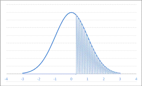
It might be useful, when thinking about Normal distributions, to consider much of the work as just a change of measurement units along the x-axis. A Standard Normal (with zero mean and standard deviation of one) can be thought of as just a change of units away from a Normal (with some non-zero mean and standard deviation other than one).
For example, the question, " For a Normal Distribution with mean 4 and standard deviation 6, what is area to the left of 1?" We can graph this as:

or it can be equivalently graphed with a change of units, by subtracting the mean (4) and dividing by the standard deviation (6):
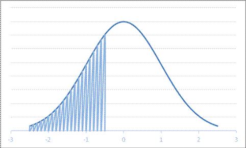
It's the same area under either distribution – it doesn't matter whether we use the red units or the blue units; we get the same answer. The blue units are "standardized" while the red are not; for the blue units we use a standard normal distribution while for the red units we use a normal distribution with a different mean and standard deviation.
- Calculate the probability in the following areas under the Standard Normal pdf with mean of zero and standard deviation of one. You might usefully draw pictures as well as making the calculations. For the calculations you can use either a computer or a table.
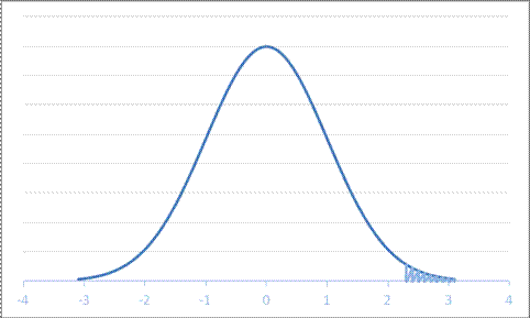
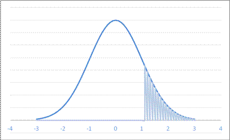
- For a Normal Distribution with mean 1 and standard deviation 9.6, what is area to the right of 23.1?
A. 0.1251 B. 0.0107 C. 0.4585 D. 0.9893
Sketch this as
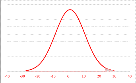
or
So, with Excel, either find the red-unit area as 1 – NORMDIST(23.1,1,9.6,TRUE) = .0107 or blue-unit area as 1 – NORMSDIST( (23.1 – 1)/9.6 ) = .0107.
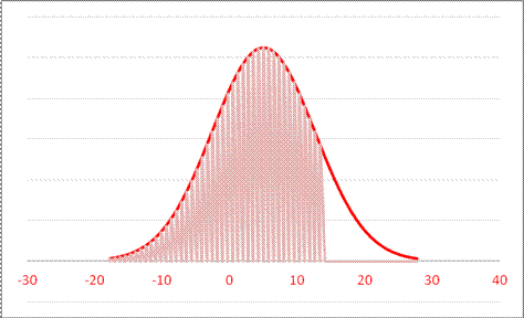
- For a Normal Distribution with mean 12 and standard deviation 7.9, what is area to the right of 30.2?
A. 0.1587 B. 0.9893 C. 0.9356 D. 0.0107
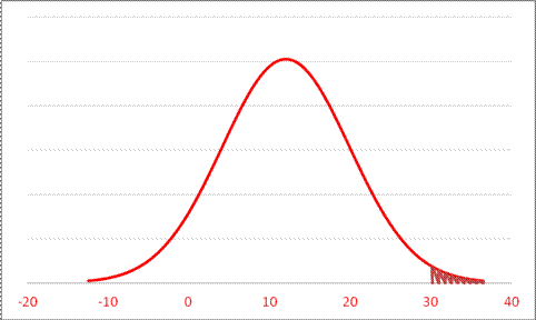
or
so .0107.
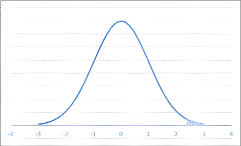
- For a Normal Distribution with mean 5 and standard deviation 7.6, what is area to the left of 14.1?
A. 0.2743 B. 0.1587 C. 0.8849 D. 0.2301
or
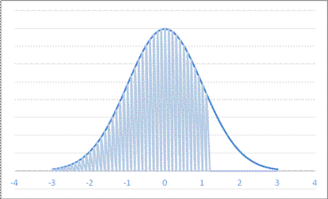
so 88%.
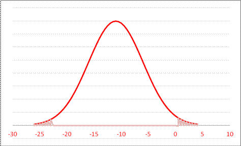
- For a Normal Distribution with mean -14 and standard deviation 2.8, what is area to the left of -20.4?
A. 0.0107 B. 0.8235 C. 0.0214 D. 0.0971
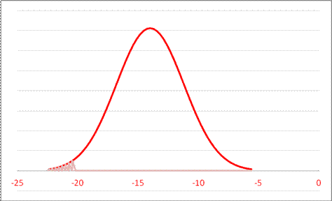
or
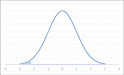
which is .0111 (not one of the answers listed, sorry!)
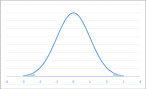
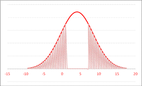
- For a Normal Distribution with mean 4 and standard deviation 7.1, what is area in both tails farther from the mean than 13.2?
A. 0.1936 B. 0.3872 C. 0.2866 D. 0.1587
or
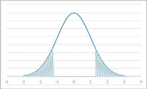
so 19%.
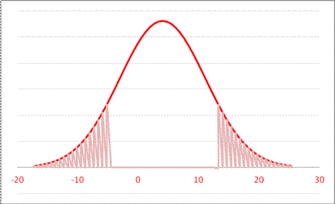
- For a Normal Distribution with mean -11 and standard deviation 5.0, what is area in both tails farther from the mean than 0.5?
A. 0.1251 B. 0.1587 C. 0.0429 D. 0.0214
or
so 2.14%.
- For a Normal Distribution with mean 11 and standard deviation 0.8, what value leaves probability 0.400 in the right tail?
A. 11.6733 B. 10.8987 C. 10.7973 D. 11.2027
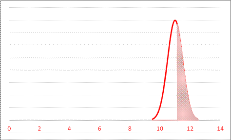
or
So 11.2 leaves 40% in the right-hand tail.
- For a Normal Distribution with mean -10 and standard deviation 2.6, what value leaves probability 0.146 in the right tail?
A. 1.0537 B. -4.8999 C. -7.2603 D. 0.8540
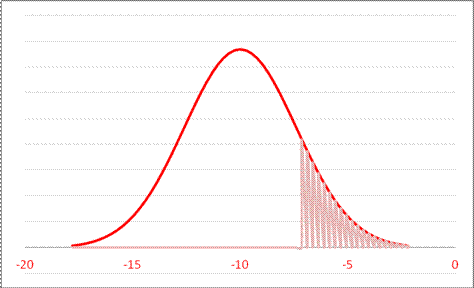
or
so -7.26 leaves 14.6 in the right tail.
- For a Normal Distribution with mean 4 and standard deviation 4.5, what values leaves probability 0.547 in both tails?
or
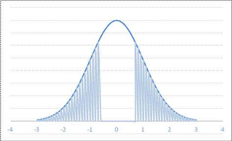
so this is the interval outside of (1.29,6.71) in red measure or ±.602 in blue measure.