Homework #4

Due Tuesday Oct 4, 2011 (that Tuesday follows a Friday schedule at CUNY!)

Econ B2000, MA Econometrics

Kevin R Foster, CCNY

For this exercise your study group may hand in a single assignment. When submitting assignments, please include your name and the assignment number as part of the filename. Please write the names of your study group members at the beginning of your homework. These assignments will be made public and available to all members of the class.

1. Who are the people in your study group?

2. What topic do you think you would like to have for your final project? Find another academic article and write a short (about a page) review. (One article per person so a 3-person study group would write 3 reviews of 3 articles.)

3. Read the section below on "Jumping into OLS" and run a linear regression with the person's income (weekly earnings) as the dependent variable. (Be careful how you restrict the sample! Should you look at everybody, or those in the labor force, or those working fulltime?) For the independent variables include at least Age, ed_HS, ed_somcoll, ed_coll, ed_advdegree, female, African-American, Asian, Native American/Indian, and Hispanic. Discuss these estimates. Then create two additional specifications with additional explanatory variables; discuss.

Jumping into OLS

OLS is Ordinary Least Squares, which as the name implies is ordinary, typical, common – something that is widely used (and abused) in just about every economic analysis.

We are accustomed to looking at graphs that show values of two variables and trying to discern patterns. Consider these two graphs of financial variables.

This plots the returns of Hong Kong's Hang Seng index against the returns of Singapore's Straits Times index (over the period from Jan 2, 1991 to Jan 31, 2006)

This next graph shows the S&P 500 returns and interest rates (1-month Eurodollar) during 1989-2004.

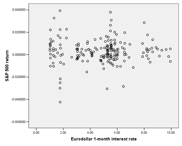
You don't have to be a highly-skilled econometrician to see the difference in the relationships. It would seem reasonable that the Hong Kong and Singapore stock indexes are closely linked while the US stock index is not closely related to interest rates.

How can we measure the relationship?

Facing a graph like the Hong Kong/Singapore stock indexes, we might represent the relationship by drawing a line, something like this:

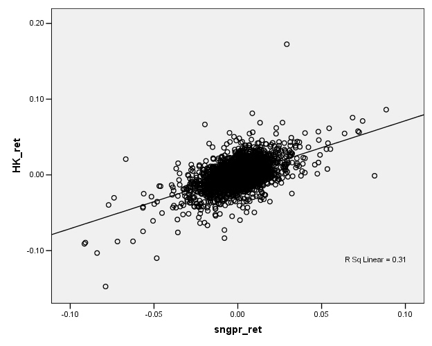
Now if this line-drawing were done just by hand, just sketching in a line, then different people would sketch different lines, which would be clearly unsatisfactory. What is the process by which we sketch the line?

Typically we want to find a relationship because we want to predict something, to find out that, if I know one variable, then how does this knowledge affect my prediction of some other variable. We call the first variable, the one known at the beginning, X. The variable that we're trying to predict is called Y. So in the example above, the Singapore stock index is X and the Hong Kong index is Y. The line that we would draw in the picture would represent our best guess of what Y would be, given our knowledge about X.

This line is drawn to get the best guess "close to" the actual Y values – where by "close to" we actually minimize the average squared distance. Why square the distance? This is one question which we will return to, again and again; for now the reason is that a squared distance really penalizes the big misses. If I square a small number, I get a bigger number. If I square a big number, I get a HUGE number. (And if I square a number less than one, I get a smaller number.) So minimizing the squared distance will mean that I am willing to make a bunch of small errors in order to reduce a really big error. This is why there is the "LS" in "OLS" -- "Ordinary Least Squares" finds the least squared difference.

A computer can easily calculate a line that minimizes the squared distance between each Y value and the best prediction. There are also formulas for it.

This is the case for the S&P 500 return and interest rates:

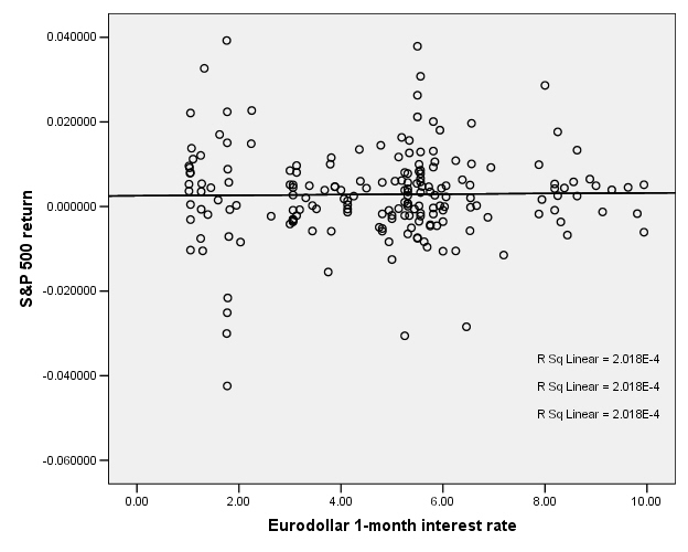
So there does not appear to be any relationship.

On SPSS

From "Analyze" choose "Regression" then "Linear". The Y-variable goes in the top box (labeled "Dependent"). Then the X-variables go into the next box (labeled "Independent").

You'll get output that looks something like this:

Coefficients^a
Model		Unstandardized Coefficients		Standardized Coefficients	t	Sig.
		B	Std. Error	Beta
1	(Constant)	35000	949.184		37.365	.000
	Edited: age	500	16.882	.104	29.122	.000
	Education High School Diploma	20000	809.111	.146	25.332	.000
	Education some college	30000	796.344	.248	41.834	.000
	Education 4-yr college degree	60000	833.640	.459	80.625	.000
	Education advanced degree	90000	936.574	.515	100.909	.000
	Female	-30000	429.340	-.247	-70.253	.000
	African-American	-9000	659.983	-.049	-13.924	.000
	Asian	2000	1204.747	.007	1.842	.066
	Native American Indian	-5000	1680.523	-.011	-3.101	.002
	Hispanic	-6000	672.377	-.037	-10.047	.000
a. Dependent Variable: Weekly earnings (2 implied decimals)

Ignore the column labeled "Standardized coefficients Beta". The "Unstandardized B" is the slope coefficient estimate and "Std. Error" is its error. The column "t" is the t-statistic and "Sig." gives the p-value.