|
Lecture Notes 2 Econ B2000, MA Econometrics Kevin R Foster, CCNY Fall 2011 |
|
|
Two Variables
In a case where we have two variables, X and Y, we want to know how or if they are related, so we use covariance and correlation.
Suppose we have a simple case where X has a two-part distribution that depends on another variable, Y. Suppose that Y is what we call a "dummy" variable: it is either a one or a zero but cannot have any other value. (Dummy variables are often used to encode answers to simple "Yes/No" questions where a "Yes" is indicated with a value of one and a "No" corresponds with a zero. Dummy variables are sometimes called "binary" or "logical" variables.) X might have a different mean depending on the value of Y.
There are millions of examples of different means between two groups. GPA might be considered, with the mean depending on whether the student is a grad or undergrad. Or income might be the variable studied, which changes depending on whether a person has a college degree or not. You might object: but there are lots of other reasons why GPA or income could change, not just those two little reasons – of course! We're not ruling out any further complications; we're just working through one at a time.
In the PUMS data, X might be "wage and salary income in past 12 months" and Y would be male or female. Would you expect that the mean of X for men is greater or less than the mean of X for women?
Run this on SPSS ...
In a case where X has two distinct distributions depending on whether the dummy variable, Y, is zero or one, we might find the sample average for each part, so calculate the average when Y is equal to one and the average when Y is zero, which we denote . These are called conditional means since they give the mean, conditional on some value.
In this case the value of is the same as the average of .
.
This is because the value of anything times zero is itself zero, so the term drops out. While it is easy to see how this additional information is valuable when Y is a dummy variable, it is a bit more difficult to see that it is valuable when Y is a continuous variable – why might we want to look at the multiplied value, ?
Use Your Eyes
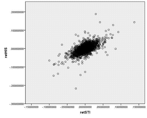
We are accustomed to looking at graphs that show values of two variables and trying to discern patterns. Consider these two graphs of financial variables.
This plots the returns of Hong Kong's Hang Seng index
against the returns of
This next graph shows the S&P 500 returns and interest rates (1-month Eurodollar) during Jan 2, 1990 – Sept 1, 2010.
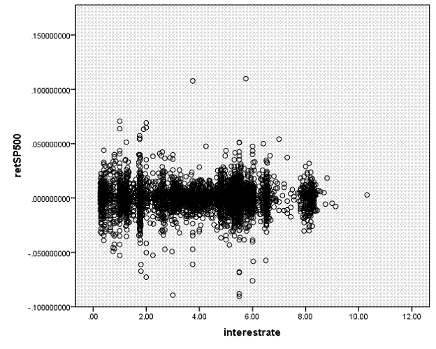
You don't have to be a highly-skilled econometrician to see
the difference in the relationships. It
would seem reasonable to state that the Hong Kong and
We want to ask, how could we measure these relationships? Since these two graphs are rather extreme cases, how can we distinguish cases in the middle? And then there is one farther, even more important question: how can we try to guard against seeing relationships where, in fact, none actually exist? The second question is the big one, which most of this course (and much of the discipline of statistics) tries to answer. But start with the first question.
How can we measure the relationship?
Correlation measures how/if two variables move together.
Recall from above that we looked at the average of when Y was a dummy variable taking only the values of zero or one. Return to the case where Y is not a dummy but is a continuous variable just like X. It is still useful to find the average of even in the case where Y is from a continuous distribution and can take any value, . It is a bit more useful if we re-write X and Y as differences from their means, so finding:
.
This is the covariance, which is denoted cov(X,Y) or sXY.
|
A positive covariance shows that when X is above its mean, Y tends to also be above its mean (and vice versa) so either a positive number times a positive number gives a positive or a negative times a negative gives a positive.
A negative covariance shows that when X is above its mean, Y tends to be below its mean (and vice versa). So when one is positive the other is negative, which gives a negative value when multiplied.
|
A bit of math (extra): = = = = =
(a strange case because it makes FOIL look like just FL!) |
Covariance is sometimes scaled by the standard deviations of X and Y in order to eliminate problems of measurement units, so the correlation is:
or Corr(X,Y),
where the Greek letter "rho" denotes the correlation coefficient. With some algebra you can show that ρ is always between negative one and positive one; .
Two variables will have a perfect correlation if they are identical; they would be perfectly inversely correlated if one is just the negative of the other (assets and liabilities, for example). Variables with a correlation close to one (in absolute value) are very similar; variables with a low or zero correlation are nearly or completely unrelated.
Sample covariances and sample correlations
Just as with the average and standard deviation, we can estimate the covariance and correlation between any two variables. And just as with the sample average, the sample covariance and sample correlation will have distributions around their true value.
Go back to the case of the Hang Seng/Straits Times stock indexes. We can't just say that when one is big, the other is too. We want to be a bit more precise and say that when one is above its mean, the other tends to be above its mean, too. We might additionally state that, when the standardized value of one is high, the other standardized value is also high. (Recall that the standardized value of one variable, X, is , and the standardized value of Y is .)
Multiplying the two values together, , gives a useful indicator since if both values are positive then the multiplication will be positive; if both are negative then the multiplication will again be positive. So if the values of ZX and ZY are perfectly linked together then multiplying them together will get a positive number. On the other hand, if ZX and ZY are oppositely related, so whenever one is positive the other is negative, then multiplying them together will get a negative number. And if ZX and ZY are just random and not related to each other, then multiplying them will sometimes give a positive and sometimes a negative number.
Sum up these multiplied values and get the (population) correlation, .
This can be written as . The population correlation between X and Y is denoted ; the sample correlation is . Again the difference is whether you divide by N or (N – 1). Both correlations are always between -1 and +1; .
We often think of drawing lines to summarize relationships; the correlation tells us something about how well a line would fit the data. A correlation with an absolute value near 1 or -1 tells us that a line (with either positive or negative slope) would fit well; a correlation near zero tells us that there is "zero relationship."
The fact that a negative value can infer a relationship might seem surprising but consider for example poker. Suppose you have figured out that an opponent makes a particular gesture when her cards are no good – you can exploit that knowledge, even if it is a negative relationship. In finance, if a fund manager finds two assets that have a strong negative correlation, that one has high returns when the other has low returns, then again this information can exploited by taking offsetting positions.
You might commonly see a "covariance matrix" if you were working with many variables; the matrix shows the covariance (or correlation) between each pair. So if you have 4 variables, named (unimaginatively) X1, X2, X3, and X4, then the covariance matrix would be:
|
|
X1 |
X2 |
X3 |
X4 |
|
X1 |
s11 |
|
|
|
|
X2 |
s21 |
s22 |
|
|
|
X3 |
s31 |
s32 |
s33 |
|
|
X4 |
s41 |
s42 |
s34 |
s44 |
Where the matrix is "lower triangular" because cov(X,Y)=cov(Y,X) [return to the formulas if you're not convinced] so we know that the upper entries would be equal to their symmetric lower-triangular entry (so the upper triangle is left blank since the entries would be redundant). And we can also show [again, a bit of math to try on your own] that cov(X,X) = var(X) so the entries on the main diagonal are the variances.
If we have a lot of variables (15 or 20) then the covariance matrix can be an important way to easily show which ones are tightly related and which ones are not.
As a practical matter, sometimes perfect (or very high) correlations can be understood simply by definition: a survey asking "Do you live in a city?" and "Do you live in the countryside?" will get a very high negative correlation between those two questions. A firm's Assets and Liabilities ought to be highly correlated. But other correlations can be caused by the nature of the sampling.
Higher Moments
The third moment is usually measured by skewness, which is a common characteristic of financial returns: there are lots of small positive values balanced by fewer but larger negative values. Two portfolios could have the same average return and same standard deviation, but if one is not symmetric distribution (so has a non-zero skewness) then it would be important to understand this risk.
The fourth moment is kurtosis, which measures how fat the tails are, or how fast the probabilities of extreme values die off. Again a risk manager, for example, would be interested in understanding the differences between a distribution with low kurtosis (so lots of small changes) versus a distribution with high kurtosis (a few big changes).
If these measures are not perfectly clear to you, don't get frustrated – it is difficult, but it is also very rewarding. As the Financial Crisis has shown, many top risk managers at name-brand institutions did not understand the statistical distributions of the risks that they were taking on. They plunged the global economy into recession and chaos because of it.
These are called "moments" to reflect the origin of the average as being like weights on a lever or "moment arm". The average is the first moment, the variance is the second, skewness is third, kurtosis is fourth, etc. If you take a class using Calculus to go through Probability and Statistics, you will learn moment-generating functions.
More examples of correlation:
It is common in finance to want to know the correlation between returns on different assets.
First remember the difference between the returns and the level of an asset or index!
An investment in multiple assets, with the same return but that are uncorrelated, will have the same return but with less overall risk. We can show this on Excel; first we'll do random numbers to show the basic idea and then use specific stocks.
How can we create normally-distributed random numbers in Excel? RAND() gives random numbers between zero and one; NORMSINV(RAND()) gives normally distributed random numbers. (If you want variables with other distributions, use the inverse of those distribution functions.) Suppose that two variables each have returns given as 2% + a normally-distributed random number; this is shown in Excel sheet, lecturenotes3.xls
With finance data, we use the return not just the price. This is because we assume that investors care about returns per dollar not the level of the stock price.
|
Important Questions |
|
|
· When we calculate a correlation, what number is "big"? Will see random errors – what amount of evidence can convince us that there is really a correlation?
· When we calculate conditional means, and find differences between groups, what difference is "big"? What amount of evidence would convince us of a difference?
To answer these, we need to think about randomness – in other perceptual problems, what would be called noise or blur.
Learning Outcomes (from CFA exam Study Session 2, Quantitative Methods)
Students will be able to:
§ calculate and interpret relative frequencies, given a frequency distribution, and describe the properties of a dataset presented as a histogram;
§ define, calculate, and interpret measures of central tendency, including the population mean, sample mean, median, and mode;
§ define, calculate, and interpret measures of variation, including the population standard deviation and the sample standard deviation;
§ define and interpret the covariance and correlation;
§ define a random variable, an outcome, an event, mutually exclusive events, and exhaustive events;
§ distinguish between dependent and independent events;
|
Probability |
|
|
Beyond presenting some basic measures such as averages and standard deviations, we want to try to understand how much these measures can tell us about the larger world. How likely is it, that we're being fooled, into thinking that there's a relationship when actually none exists? To think through these questions we must consider the logical implications of randomness and often use some basic statistical distributions (discrete or continuous).
Think Like a Statistician
The basic question that a Statistician must ask is "How likely is it, that I'm being fooled?" Once we accept that the world is random (rather than a manifestation of some god's will), we must decide how to make our decisions, knowing that we cannot guarantee that we will always be right. There is some risk that the world will seem to be one way, when actually it is not. The stars are strewn randomly across the sky but some bright ones seem to line up into patterns. So too any data might sometimes line up into patterns.
Statisticians tend to stand on their heads and ask, suppose there were actually no relationship? (Sometimes they ask, "suppose the conventional wisdom were true?") This statement, about "no relationship," is called the Null Hypothesis, sometimes abbreviated as H0. The Null Hypothesis is tested against an Alternative Hypothesis, HA.
Before we even begin looking at the data we can set down some rules for this test. We know that there is some probability that nature will fool me, that it will seem as though there is a relationship when actually there is none. The statistical test will create a model of a world where there is actually no relationship and then ask how likely it is that we could see what we actually see, "How likely is it, that I'm being fooled?" What if there were actually no relationship, is there some chance that I could see what I actually see?
Randomness in Sports
As an example, consider sports events. As any sports fan knows, a team or individual can get lucky or unlucky. The baseball World Series, for example, has seven games. It is designed to ensure that, by the end, one team or the other wins. But will the better team always win?
First make a note about subjectivity: if I am a fan of the team that won, then I will be convinced that the better team won; if I'm a fan of the losing team then I'll be certain that the better team got unlucky. But fans of each team might agree, if they discussed the question before the Series were played, that luck has a role.
Will the better team win? Clearly a seven-game Series means that one team or the other will win, even if they are exactly matched (if each had precisely a 50% chance of winning). If two representatives tossed a coin in the air seven times, then one or the other would win at least four tosses – maybe even more. We can use a computer to simulate seven coin-tosses by having it pick a random number between zero and one and defining a "win" as when the random number is greater than 0.5.
Or instead of having a computer do it, we could use a bit of statistical theory.
Some math
Suppose we start with just one coin-toss or game (baseball uses 7 games to decide a champion; football uses just one). Choose to focus on one team so that we can talk about "win" and "loss". If this team has a probability of winning that is equal to p, then it has a probability of losing equal to (1-p). So even if p, the probability of winning, is equal to 0.6, there is still a 40% chance that it could lose a single game. In fact unless the probability of winning is 100%, there is some chance, however remote, that the lesser team will win.
What about if they played two games? What are the outcomes? The probability of a team winning both games is p*p = p2. If the probability were 0.5 then the probability of winning twice in a row would be 0.25.
A table can show this:
|
|
Win Game 1 {p} |
Lose Game 1 {1-p} |
|
Win Game 2 {p} |
outcome: W,W |
L,W |
|
Lose Game 2 {1-p} |
W,L |
L,L |
This is a fundamental fact about how probabilities are represented mathematically: if the probabilities are not related (i.e. if the tossed coin has no memory) then the probability of both events happening is found my multiplying the probabilities of each individual outcome. (What if they're not unrelated, you may ask? What if the first team that wins gets a psychological boost in the next so they're more likely to win the second game? Then the math gets more complicated – we'll come back to that question!)
The math notation for two events, call them A and B, both happening is:
The fundamental fact of independence is then represented as:
where we use the term "independent" for when there is no relationship between them.
The probability that a team could lose both games is (1-p)*(1-p) = (1-p)2. The probability that the teams could split the series (each wins just one) is p*(1-p) + (1-p)*p = 2p(1-p). There are two ways that each team could win just one game: either the series splits (Win,Loss) or (Loss,Win).
For three games the outcomes become more complicated: now there are 8 combinations of win and loss:
|
(W,W,W) |
(W,W,L) |
(W,L,W) |
(L,W,W) |
(W,L,L) |
(L,W,L) |
(L,L,W) |
(L,L,L) |
|
p*p*p |
p*p*(1-p) |
p*(1-p)p |
(1-p)p*p |
p(1-p)(1-p) |
(1-p)p(1-p) |
(1-p)(1-p)p |
(1-p)(1-p)(1-p) |
and the probabilities are in the row below.
The team will win the series in any of the left-most 4 outcomes so its overall probability of winning the series is
while its probability of losing the series is
.
Clearly if p is 0.5 so that p=(1-p) then the chances of either team winning the three-game series are equal. If the probabilities are not equal then the chances are different, but as long as there is a probability not equal to one or zero (i.e. no certainty) then there is a chance that the worse team could win.
If you keep on working out the probabilities for longer and longer series you might notice that the coefficients and functional forms are right out of Pascal's Triangle. This is your first notice of just how "normal" the Normal Distribution is, in the sense that it jumps into all sorts of places where you might not expect it. The terms of Pascal's Triangle begin (as N becomes large) to have a normal distribution! We'll come back to this again...
Terms and Definitions
Some basics: a sample space is the entire list of possible outcomes (can be whole long list or even mathematical sets such as real numbers); events are subsets of the sample space. Simple event is a single outcome (one dice comes up 6); a compound event is several outcomes (both dice come up 6). Notate an event as A. The complement of the event is the set of all events that are not in A; this is A'.
The events must be mutually exclusive and exhaustive, so a good deal of the hard work in probability is just figuring out how to list all of the events.
Mutually exclusive means that the events must be clearly defined so that the data observed can be classified into just one event. Exhaustive means that every possible data observed must fit into some event. The "mutually exclusive" part means that probabilities can be added up, so that if the probability of rolling a "1" on a dice is 1/6 and the probability of rolling a 6 is 1/6, then the probability of rolling either a 1 or 6 is 2/6 = 1/3. The "exhaustive" part of defining the events means that the sum of all the events must equal one.
For example, suppose we roll two dice. We might want to think of "die #1 comes up as 6" as one event [in English, the singular of "dice" is "die" – how morbid gambling can be!]. But the other die can have 6 different values without changing the value of the first die. So a better list of events would be the integers from 2 to 12, the sum of the dice values – with the note that there are many ways of achieving some of the events (a 7 is a 6 &1 or a 5&2, or 4&3, or 3&4, or 2&5, or 1&6) while other events have only one path (each die comes up 6 to make 12).
A sample space is the set of all possible events. The sum of the probability of all of the events in the sample space is equal to one. There is a 100% chance that something happens (provided we've defined the sample space correctly). So if a lottery brags that there is a 2% chance that "you might be a winner!" this is equivalent to stating that there is a 98% chance that you'll lose.
Events have probability; this must lie between zero and one (inclusive); so . The probability of all of the events in the sample space must sum to one. This means that the probability of an event and its complement must sum to one: .
Probabilities come from empirical results (relative frequency approach) or the classical (a priori or postulated) assignment or from subjective beliefs that people have.
In empirical approach, the Law of Large Numbers is important: as the number of identical trials increases, the estimated frequency approaches its theoretical value. You can try flipping coins and seeing how many come up heads (flip a bunch at a time to speed up the process); it should be 50%.
We are often interested in finding the probability of two events both happening; this is the "intersection" of two events; the logical "and" relationship; two things both occurring. In the PUMS data we might want to find how many females have a college degree; in poker we might care about the chance of an opponent having an ace as one of her hole cards and the dealer turning up a king. We notate the intersection of A and B as and want to find . In SPSS this is notated with "&".
The "union" of two events is the logical "or" so it is either of two events occurring; this is so we might consider or, in SPSS, "|". In the PUMS data we might want to combine people who report themselves as having race "black" with those who report "black – white". In cards, it is the probability that any of my 3 opponents has a better hand.
Married people can buy life insurance policies that pay out either when the first person dies or after both die – logical and vs or.
Venn Diagrams (Ballantine)

General Law of Addition
and so
Mutually Exclusive (Special Law of Addition),
If then and
Conditional Probability
if . See Venn Diagram.
Independent Events
A is independent of B if and only if
If we have multiple random variables then we can consider their Joint Distribution: the probability associated with each outcome in both sample spaces. So a coin flip has a simple discrete distribution: a 50% chance of heads and a 50% chance of tails. Flipping 2 coins gives a joint distribution: a 25% chance of both coming up heads, a 25% chance of both coming up tails, and a 50% chance of getting one head and one tail.
The probability of multiple independent events is found by multiplying the probabilities of each event together. So the chance of rolling two 6 on two dice is . The probability of getting to the computer lab on the 6th floor of NAC from the first floor, without having to walk up a broken escalator, can be found this way too. Suppose the probability of an escalator not working is ; then the probability of it working is and the probability of five escalators each working is . So even if the probability of a breakdown is small (5%), still the probability of having every escalator work is just so this implies that you'd expect to walk more than once a week.
A simple representation of the joint distribution of two coin flips is a table:
|
|
coin 1 Heads |
coin 1 Tails |
|
coin 2 Heads |
H,H at 25% |
H,T at 25% |
|
coin 2 Tails |
T,H at 25% |
T,T at 25% |
Where, since the outcomes are independent, we can just multiply the probabilities.
The Joint Distribution tells the probabilities of all of the different outcomes. A Marginal Distribution answers a slightly different question: given some value of one of the variables, what are the probabilities of the other variables?
When the variables are independent then the marginal distribution does not change from the joint distribution. Consider a simple example of X and Y discrete variables. X takes on values of 1 or 2 with probabilities of 0.6 and 0.4 respectively. Y takes on values of 1, 2, or 3 with probabilities of 0.5, 0.3, and 0.2 respectively. So we can give a table like this:
|
|
X=1 (60%) |
X=2 (40%) |
|
|
Y=1 (50%) |
(1,1) at probability 0.3 |
(2,1) at probability 0.2 |
|
|
Y=2 (30%) |
(1,2) at probability 0.18 |
(2,2) at probability 0.12 |
|
|
Y=3 (20%) |
(1,3) at probability 0.12 |
(2,3) at probability 0.08 |
|
|
|
|
|
|
On the assumption that X and Y are independent. The probabilities in each box are found by multiplying the probability of each independent event.
If instead we had the two variables, A and B, not being independent then we might have a table more like this:
|
|
A=1 |
A=2 |
|
|
B=1 |
(1,1) at probability 0.25 |
(2,1) at probability 0.13 |
|
|
B=2 |
(1,2) at probability 0.23 |
(2,2) at probability 0.12 |
|
|
B=3 |
(1,3) at probability 0.17 |
(2,3) at probability 0.1 |
|
|
|
|
|
|
We will examine the differences.
If we add up the probabilities along either rows or columns then we get the marginal probabilities (which we write in the margins, appropriately enough). Then we'd get:
|
|
X=1 (60%) |
X=2 (40%) |
|
|
Y=1 (50%) |
(1,1) at probability 0.3 |
(2,1) at probability 0.2 |
0.5 |
|
Y=2 (30%) |
(1,2) at probability 0.18 |
(2,2) at probability 0.12 |
0.3 |
|
Y=3 (20%) |
(1,3) at probability 0.12 |
(2,3) at probability 0.08 |
0.2 |
|
|
0.6 |
0.4 |
|
Which just re-states our assumption that the variables are independent – and shows that, where there is independence, the probability of either variable alone does not depend on the value that the other variable takes on. In other words, knowing X does not give me any information about the value that Y will take on, and vice versa.
If instead we do this for the A,B case we get:
|
|
A=1 |
A=2 |
|
|
B=1 |
(1,1) at probability 0.25 |
(2,1) at probability 0.13 |
0.38 |
|
B=2 |
(1,2) at probability 0.23 |
(2,2) at probability 0.12 |
0.35 |
|
B=3 |
(1,3) at probability 0.17 |
(2,3) at probability 0.1 |
0.27 |
|
|
0.65 |
0.35 |
|
Where we double check that we've done it right by seeing that the sum of either of the marginals is equal to one (65% + 35% = 100% and 38% + 35% + 27% = 100%).
So the marginal distributions sum the various ways that an outcome can happen. For example, we can get A=1 in any of 3 ways: either (1,1), (1,2) or (1,3). So we add the probabilities of each of these outcomes to find the total chance of getting A=1.
But if we want to understand how A and B are related, it might be more useful to consider this as a prediction problem: would knowing the value that A takes on help me guess the value of B? Would knowing the value that B takes on help me guess the value of A?
These are abstract questions but they have vitally important real-life analogs. In airport security, is the probability that someone is a terrorist independent of whether they are Muslim? Is the probability that someone is pulled out of line for a thorough search independent of whether they are Muslim? (The TSA might have different beliefs than you or me!) In medicine, is the probability that someone gets cancer independent of whether they eat lots of vegetables? In economics, is the probability that someone defaults on their mortgage independent of the mortgage originator (Fannie, Freddie, mortgage broker, bank)? Is the probability of the country pulling out of recession independent of whether the Fed raises rates? In poker, if my opponent just raised the bid, what is the probability that her cards are better than mine?
For these questions we want to find the conditional distribution: what is the probability of some outcome, given a particular value for some other random variable?
Just from the phrasing of the question, you should be able to see that if the two variables are independent then the conditional distribution should not change from the marginal distribution – as is the case of X and Y. Flipping a coin does not help me guess the outcome of a roll of the dice. (Cheering in front of a sports game on TV does not affect the outcome, for another example – although plenty of people act as though they don't believe that!)
How do we find the conditional distribution? Take the value of the joint distribution and divide it by the marginal distribution of the relevant variable.
For example, suppose we want to find the probability of B outcomes, conditional on A=1. Since we know that A=1, there is no longer a 65% probability of A -- it happened. So we divide each joint probability by 0.65 so that the sum will be equal to 1. So the probabilities are now:
|
|
A=1 |
A=2 |
|
|
B=1 |
(1,1) at probability 0.25/.65 |
(2,1) at probability 0.13 |
0.38 |
|
B=2 |
(1,2) at probability 0.23/.65 |
(2,2) at probability 0.12 |
0.35 |
|
B=3 |
(1,3) at probability 0.17/.65 |
(2,3) at probability 0.1 |
0.27 |
|
|
0.65/.65 |
0.35 |
|
so now we get the conditional distribution:
|
|
A=1 |
A=2 |
|
|
B=1 |
(1,1) @ 0.3846 |
(2,1) at probability 0.13 |
0.38 |
|
B=2 |
(1,2) @ 0.3538 |
(2,2) at probability 0.12 |
0.35 |
|
B=3 |
(1,3) @ 0.2615 |
(2,3) at probability 0.1 |
0.27 |
|
|
|
0.35 |
|
We could do the same to find the conditional distribution of B, given that A=2:
|
|
A=1 |
A=2 |
|
|
B=1 |
(1,1) at probability 0.25 |
(2,1) @ 0.13/.35 =.3714 |
0.38 |
|
B=2 |
(1,2) at probability 0.23 |
(2,2) @ 0.12/.35 = .3429 |
0.35 |
|
B=3 |
(1,3) at probability 0.17 |
(2,3) @ 0.1/.35 = .2857 |
0.27 |
|
|
0.65 |
|
|
These conditional probabilities are denoted as for example. We could find the expected value of B given that A equals 2, , just by multiplying the value of B by its probability of occurrence, so .
We could find the conditional probabilities of A given B=1 or given B=2 or given B=3. In those cases we would sum across the rows rather than down the columns.
More pertinently, we can get crosstabs (on SPSS, "Analyze" then "Descriptive Statistics" then "Crosstabs") on two variables, for example the native/foreign born in each borough,
|
|
|
foreign_born |
Total |
|
|
|
|
0 |
1 |
|
|
boroughs |
Bronx |
33955 |
15928 |
49883 |
|
Manhattan |
40511 |
15632 |
56143 |
|
|
Staten Is |
16074 |
3971 |
20045 |
|
|
Brooklyn |
62464 |
37324 |
99788 |
|
|
Queens |
48193 |
41719 |
89912 |
|
|
Total |
201197 |
114574 |
315771 |
|
To get the joint probabilities, we divide the counts by the grand total,
|
native |
foreign |
|
|
Bronx |
0.1075 |
0.0504 |
|
Manhattan |
0.1283 |
0.0495 |
|
Staten Is |
0.0509 |
0.0126 |
|
Brooklyn |
0.1978 |
0.1182 |
|
Queens |
0.1526 |
0.1321 |
Then get the marginals:
|
native |
foreign |
||
|
Bronx |
0.1075 |
0.0504 |
0.1580 |
|
Manhattan |
0.1283 |
0.0495 |
0.1778 |
|
Staten Is |
0.0509 |
0.0126 |
0.0635 |
|
Brooklyn |
0.1978 |
0.1182 |
0.3160 |
|
Queens |
0.1526 |
0.1321 |
0.2847 |
|
0.6372 |
0.3628 |
These show that, in NYC, 64% are natives and 36% are foreign-born. The most populous boroughs are Brooklyn and Queens, each with about 30% of the city's population, while Manhattan and the Bronx each have about 15% and tiny Staten Island has just over 6%.
Then the conditional probabilities. Conditional on being native born,
|
native |
foreign |
||
|
Bronx |
0.1688 |
0.0504 |
0.1580 |
|
Manhattan |
0.2013 |
0.0495 |
0.1778 |
|
Staten Is |
0.0799 |
0.0126 |
0.0635 |
|
Brooklyn |
0.3105 |
0.1182 |
0.3160 |
|
Queens |
0.2395 |
0.1321 |
0.2847 |
|
0.6372 |
0.3628 |
So 31% of the natives live in Brooklyn, 24% in Queens, 20% in Manhattan, 17% in the Bronx, and 8% in Staten Island. So a larger fraction of natives (relative to overall population share) is in Manhattan and Staten Island while a much lower fraction of native-born are in Queens.
Conditional on being foreign born,
|
native |
foreign |
||
|
Bronx |
0.1075 |
0.1390 |
0.1580 |
|
Manhattan |
0.1283 |
0.1364 |
0.1778 |
|
Staten Is |
0.0509 |
0.0347 |
0.0635 |
|
Brooklyn |
0.1978 |
0.3258 |
0.3160 |
|
Queens |
0.1526 |
0.3641 |
0.2847 |
|
0.6372 |
0.3628 |
So 36% of immigrants live in Queens (relative to 28% of the population overall), 33% in Brooklyn, 14% in the Bronx and Manhattan, and just 3% in Staten Island.
The relative fractions of native/immigrant by borough (so conditional probabilities) is
|
native |
foreign |
||
|
Bronx |
0.6807 |
0.3193 |
0.1580 |
|
Manhattan |
0.7216 |
0.2784 |
0.1778 |
|
Staten Is |
0.8019 |
0.1981 |
0.0635 |
|
Brooklyn |
0.6260 |
0.3740 |
0.3160 |
|
Queens |
0.5360 |
0.4640 |
0.2847 |
|
0.6372 |
0.3628 |
So the borough with the highest fraction of immigrants is Queens (a 54-46 split), followed by Brooklyn, the Bronx, Manhattan, and Staten Island (where natives outnumber immigrants by 4-to-1).
Conditional probabilities can also be calculated with what is called Bayes' Theorem:
.
This can be understood by recalling the definition of conditional probability, , so , that the conditional probability equals the joint probability divided by the marginal probability.
The power of Bayes' Theorem can be understood by thinking about medical testing. Suppose a genetic test screens for some disease with 99% accuracy. Your test comes back positive – how worried should you be? The surprising answer is not 99% worried; in fact often you might be more than likely to be healthy! Suppose that the disease is rare so only 1 person in 1000 has it (so 0.1%). So out of 1000 people, one person has the disease and the test is 99% likely to identify that person. Out of the remaining 999 people, 1% will be misidentified as having the disease, so this is 9.99 – call it 10 people. So eleven people will test positive but only one will actually have the disease so the probability of having the disease given that the test comes up positive, , is = .
The test is not at all useless – it has brought down an individual's likelihood of being sick by orders of magnitude, from one-tenth of one percent to ten percent. But it's still not nearly as accurate as the "99%" label might imply.
Many healthcare providers don't quite get this and explain it merely as "don't be too worried until we do further tests." But this is one reason why broad-based tests can be very expensive and not very helpful. These tests are much more useful if we first narrow down the population of people who might have the disease. For example home pregnancy tests might be 99% accurate but if you randomly selected 1000 people to take the test, you'd find many false positives. Some of those might be guys (!) or women who, for a variety of reasons, are not likely to be pregnant. The test is only useful as one element of a screen that gets progressively finer and finer.
Counting Rules
If A can occur as N1 events and B can be N2 events then the sample space is (visualize a contingency table with N1 rows and N2 columns).
Factorials: If there are N items then they can be arranged in ways.
Permutations: n events that can occur in r items (where order is important) have a total of possible outcomes.
Combinations: n events that can occur in r items (where order is not important) have possible outcomes – just the permutation divided by r! to take care of the multiple ways of ordering.
So to apply these, consider computer passwords (see NYTimes article below).
The article reports:
Mr. Herley, working with Dinei Florêncio, also at Microsoft Research, looked at the password policies of 75 Web sites. ... They reported that the sites that allowed relatively weak passwords were busy commercial destinations, including PayPal, Amazon.com and Fidelity Investments. The sites that insisted on very complex passwords were mostly government and university sites. What accounts for the difference? They suggest that “when the voices that advocate for usability are absent or weak, security measures become needlessly restrictive.”
Consider the simple mathematics of why a government or university might want complex passwords. How many permutations are possible if passwords are 6 numerical digits? How many if passwords are 6 alphabetic or numeric characters? If the characters are alphabetic, numeric, and fifteen punctuation characters (, . _ - ? ! @ # $ % ^ & * ' ")? What if passwords are 8 characters? If each login attempt takes 1/100 of a second, how many seconds of "brute-force attack" does it take to access the account on average? If there is a penalty of 10 minutes after 3 unsuccessful login attempts, how long would it take to break in? (Of course, the article notes, if password requirements are so arcane that employees put their passwords on a Post-It attached to the monitor, then the calculations above are irrelevant.)