|
Lecture Notes 5 Econ B2000, MA Econometrics Kevin R Foster, CCNY Fall 2011 |
|
|
Learning Outcomes (from CFA exam Study Session 3, Quantitative Methods)
Students will be able to:
§ construct and interpret a confidence interval for a normally distributed random variable, and determine the probability that a normally distributed random variable lies inside a given confidence interval;
§ define the standard normal distribution, explain how to standardize a random variable, and calculate and interpret probabilities using the standard normal distribution;
§ explain the construction of confidence intervals;
§ define a hypothesis, describe the steps of hypothesis testing, interpret and discuss the choice of the null hypothesis and alternative hypothesis, and distinguish between one-tailed and two-tailed tests of hypotheses;
§ define and interpret a test statistic, a Type I and a Type II error, and a significance level, and explain how significance levels are used in hypothesis testing;
|
Hypothesis Testing |
|
|
One of the principal tasks facing the statistician is to perform hypothesis tests. These are a formalization of the most basic questions that people ask and analyze every day – just contorted into odd shapes. But as long as you remember the basic common sense underneath them, you can look up the precise details of the formalization that lays on top.
The basic question is "How likely is it, that I'm being fooled?" Once we accept that the world is random (rather than a manifestation of some god's will), we must decide how to make our decisions, knowing that we cannot guarantee that we will always be right. There is some risk that the world will seem to be one way, when actually it is not. The stars are strewn randomly across the sky but some bright ones seem to line up into patterns. So too any data might sometimes line up into patterns.
A formal hypothesis sets a mathematical condition that I want to test. Often this condition takes the form of some parameter being zero for no relationship or no difference.
Statisticians tend to stand on their heads and ask: What if there were actually no relationship? (Usually they ask questions of the form, "suppose the conventional wisdom were true?") This statement, about "no relationship," is called the Null Hypothesis, sometimes abbreviated as H0. The Null Hypothesis is tested against an Alternative Hypothesis, HA.
Before we even begin looking at the data we can set down some rules for this test. We know that there is some probability that nature will fool me, that it will seem as though there is a relationship when actually there is none. The statistical test will create a model of a world where there is actually no relationship and then ask how likely it is that we could see what we actually see, "How likely is it, that I'm being fooled?"
The "likelihood that I'm being fooled" is the p-value.
For a scientific experiment we typically first choose the level of certainty that we desire. This is called the significance level. This answers, "How low does the p-value have to be, for me to accept the formal hypothesis?" To be fair, it is important that we set this value first because otherwise we might be biased in favor of an outcome that we want to see. By convention, economists typically use 10%, 5%, and 1%; 5% is the most common.
A five percent level of a test is conservative, it means that we want to see so much evidence that there is only a 5% chance that we could be fooled into thinking that there's something there, when nothing is actually there. Five percent is not perfect, though – it still means that of every 20 tests where I decide that there is a relationship there, it is likely that I'm being fooled in one of those – I'm seeing a relationship where there's nothing there.
To help ourselves to remember that we can never be truly certain of our judgment of a test, we have a peculiar language that we use for hypothesis testing. If the "likelihood that I'm being fooled" is less than 5% then we say that the data allow us to reject the null hypothesis. If the "likelihood that I'm being fooled" is more than 5% then the data do not reject the null hypothesis.
Note the formalism: we never "accept" the null hypothesis. Why not? Suppose I were doing something like measuring a piece of machinery, which is supposed to be a centimeter long. The null hypothesis is that it is not defective and so is one centimeter in length. If I measure with a ruler I might not find any difference to the eye. So I cannot reject the hypothesis that it is one centimeter. But if I looked with a microscope I might find that it is not quite one centimeter! The fact that, with my eye, I don't see any difference, does not imply that a better measurement could not find any difference. So I cannot say that it is truly exactly one centimeter; only that I can't tell that it isn't.
So too with statistics. If I'm looking to see if some portfolio strategy produces higher returns, then with one month of data I might not see any difference. So I would not reject the null hypothesis (that the new strategy is no improvement). But it is possible that the new strategy, if carried out for 100 months or 1000 months or more might show some tiny difference.
Not rejecting the null is saying that I'm not sure that I'm not being fooled. (Read that sentence again; it's not immediately clear but it's trying to make a subtle and important point.)
To summarize, Hypothesis Testing asks, "What is the chance that I would see the value that I've actually got, if there truly were no relationship?" If this p-value is lower than 5% then I reject the null hypothesis of "no relationship." If the p-value is greater than 5% then I do not reject the null hypothesis of "no relationship."
The rest is mechanics.
The null hypothesis would tell that a parameter has some particular value, say zero: ; the alternative hypothesis is . Under the null hypothesis the parameter has some distribution (often normal), so . Generally we have an estimate for , which is (for small samples this inserts additional uncertainty). So I know that, under the null hypothesis, has a standard normal distribution (mean of zero and standard deviation of one). I know exactly what this distribution looks like, it's the usual bell-shaped curve:
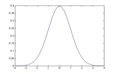
So from this I can calculate, "What is the chance that I would see the value that I've actually got, if there truly were no relationship?," by asking what is the area under the curve that is farther away from zero than the value that the data give. (I still don't know what value the data will give! I can do all of this calculation beforehand.)
Any particular estimate of is generally going to be . So the test statistic is formed with .
Looking at the standard normal pdf, a value of the test statistic of 1.5 would not meet the 5% criterion (go back and calculate areas under the curve). A value of 2 would meet the 5% criterion, allowing us to reject the null hypothesis. For a 5% significance level, the standard normal critical value is 1.96: if the test statistic is larger than 1.96 (in absolute value) then its p-value is less than 5%, and vice versa. (You can find critical values by looking them up in a table or using the computer.)
Sidebar: Sometimes you see people do a one-sided test, which is within the letter of the law but not necessarily the spirit of the law (particularly in regression formats). It allows for less restrictive testing, as long as we believe that we know that there is only one possible direction of deviation (so, for example, if the sample could be larger than zero but never smaller). But in this case maybe the normal distribution is inapplicable.
The test statistic can be transformed into measurements of or into a confidence interval.
If I know that I will reject the null hypothesis of at a 5% level if the test statistic, , is greater than 1.96 (in absolute value), then I can change around this statement to be about . This says that if the estimated value of is less than 1.96 standard errors from zero, we cannot reject the null hypothesis. So cannot reject if:
.
This range, , is directly comparable to . If I divide by its standard error then this ratio has a normal distribution with mean zero and standard deviation of one. If I don't divide then has a normal distribution with mean zero and standard deviation, .
If the null hypothesis is not zero but some other number, , then under the null hypothesis the estimator would have a normal distribution with mean of and standard error, . To transform this to a standard normal would mean subtracting the mean and dividing by , so cannot reject if , i.e. cannot reject if is within the range, .
Confidence Intervals
We can use the same critical values to construct a confidence interval for the estimator, usually expressed in the form . This shows that, for a given sample size (therefore , which depends on the sample size) that there is a 95% likelihood that the interval formed around a given estimator contains the true value.
This relates to hypothesis testing because if the confidence interval includes the null hypothesis then we cannot reject the null; if the null hypothesis value is outside of the confidence interval then we can reject the null.
Find p-values
We can also find p-values associated with a particular null hypothesis by turning around the process outlined above. If the null hypothesis is zero, then with a 5% significance level we reject the null if is greater than 1.96 in absolute value. What if the ratio were 2 – what is the smallest significance level that would still reject? (Check your understanding: is it more or less than 5%?)
We can compute the ratio and then convert this number to a p-value, which is the smallest significance level that would still reject the null hypothesis (and if the null is rejected at a low level then it would automatically be rejected at any higher levels).
Type I and Type II Errors
Whenever we use statistics we must accept that there is a likelihood of errors. In fact we distinguish between two types of errors, called (unimaginatively) Type I and Type II. These errors arise because a null hypothesis could be either true or false and a particular value of a statistic could lead me to reject or not reject the null hypothesis, H0. A table of the four outcomes is:
|
|
H0 is true |
H0 is false |
|
Do not reject H0 |
good! |
oops – Type II |
|
Reject H0 |
oops – Type I |
good! |
Our chosen significance level (usually 5%) gives the probability of making an error of Type I. We cannot control the level of Type II error because we do not know just how far away H0 is from being true. If our null hypothesis is that there is a zero relationship between two variables, when actually there is a tiny, weak relationship of 0.0001%, then we could be very likely to make a Type II error. If there is a huge, strong relationship then we'd be much less likely to make a Type II error.
There is a tradeoff (as with so much else in economics!). If I push down the likelihood of making a Type I error (using 1% significance not 5%) then I must be increasing the likelihood of making a Type II error.
Edward Gibbon notes that the emperor Valens would "satisfy his anxious suspicions by the promiscuous execution of the innocent and the guilty" (chapter 26). This rejects the null hypothesis of "innocence"; so a great deal of Type I error was acceptable to avoid Type II error.
Every email system fights spam with some sort of test: what is the likelihood that a given message is spam? If it's spam, put it in the "Junk" folder; else put it in the inbox. A Type I error represents putting good mail into the "Junk" folder; Type II puts junk into your inbox.
Examples
Let's do some examples.
Assume that the calculated average is 3, the sample standard deviation is 15, and there are 100 observations. The null hypothesis is that the average is zero. The standard error of the average is . We can immediately see that the sample average is more than two standard errors away from zero so we can reject at a 95% confidence level.
Doing this step-by-step, the average over its standard error is . Compare this to 1.96 and see that 2 > 1.96 so we can reject. Alternately we could calculate the interval, , which is = (-2.94, 2.94), outside of which we reject the null. And 3 is outside that interval. Or calculate a 95% confidence interval of , which does not contain zero so we can reject the null. The critical value for the estimate of 3 is 4.55% (found from Excel either 2*(1-NORMSDIST(2)) if using the standard normal distribution or 2*(1-NORMDIST(3,0,1.5,TRUE)) if using the general normal distribution with a mean of zero and standard error of 1.5).
If the sample average were -3, with the same sample standard deviation and same 100 observations, then the conclusions would be exactly the same.
Or suppose you find that the average difference between two samples, X and Y, (i.e. ) is -0.0378. The sample standard deviation is 0.357. The number of observations is 652. These three pieces of information are enough to find confidence intervals, do t-tests, and find p-values.
How?
First find the standard error of the average difference. This standard error is 0.357 divided by the square root of the number of observations, so .
So we know (from the Central Limit Theorem) that the average has a normal distribution. Our best estimate of its true mean is the sample average, -0.0378. Our best estimate of its true standard error is the sample standard error, 0.01398. So we have a normal distribution with mean -0.0378 and standard error 0.01398.
We can make this into a standard normal distribution by adding 0.0378 and dividing by the sample standard error, so now the mean is zero and the standard error is one.
We want to see how likely it would be, if the true mean were actually zero, that we would see a value as extreme as -0.0378. (Remember: we're thinking like statisticians!)
The value of -0.0378 is = -2.70 standard deviations from zero.
From this we can either compare this against critical t-values or use it to get a p-value.
To find the p-value, we can use Excel just like in the homework assignment. If we have a standard normal distribution, what is the probability of finding a value as far from zero as -2.27, if the true mean were zero? This is 2*(1-NORMSDIST(-2.27)) = 0.6%. The p-value is 0.006 or 0.6%. If we are using a 5% level of significance then since 0.6% is less than 5%, we reject the null hypothesis of a zero mean. If we are using a 1% level of significance then we can reject the null hypothesis of a zero mean since 0.6% is less than 1%.
Or instead of standardizing we could have used Excel's other function to find the probability in the left tail, the area less than -0.0378, for a distribution with mean zero and standard error 0.01398, so 2*NORMDIST(-0.0378,0,0.01398,TRUE) = 0.6%.
Standardizing means (in this case) zooming in, moving from finding the area in the tail of a very small pdf, like this:
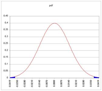
to moving to a standard normal, like this:
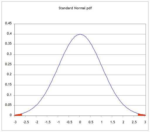
But since we're only changing the units on the x-axis, the two areas of probability are the same.
We could also work backwards. We know that if we find a standardized value greater (in absolute value) than 1.96, we would reject the null hypothesis of zero at the 5% level. (You can go back to your notes and/or HW1 to remind yourself of why 1.96 is so special.)
We found that for this particular case, each standard deviation is of size . So we can multiply 1.96 times this value to see that if we get a value for the mean, which is farther from zero than 0.01398*1.96 = 0.0274, then we would reject the null. Sure enough, our value of -0.0378 is farther from zero, so we reject.
Alternately, use this 1.96 times the standard error to find a confidence interval. Choose 1.96 for a 95% confidence interval, so the confidence interval around -0.0378 is plus or minus 0.0274, , which is the interval (-0.0652, -0.0104). Since this interval does not include zero we can be 95% confident that we can reject the null hypothesis of zero.
Complications from a Series of Hypothesis Tests
Often a modeler will make a series of hypothesis tests to attempt to understand the inter-relations of a dataset. However while this is often done, it is not usually done correctly. Recall from our discussion of Type I and Type II errors that we are always at risk of making incorrect inferences about the world based on our limited data. If a test has an significance level of 5% then we will not reject a null hypothesis until there is just a 5% probability that we could be fooled into seeing a relationship where there is none. This is low but still is a 1-in-20 chance. If I do 20 hypothesis tests to find 20 variables that significantly impact some variable of interest, then it is likely that one of those variables is fooling me (I don't know which one, though). It is also likely that my high standard of proof meant that there are other variables which are more important but which didn't seem it.
Sometimes you see very stupid people who collect a large number of possible explanatory variables, run hundreds of regressions, and find the ones that give the "best-looking" test statistics – the ones that look good but are actually entirely fictitious. Many statistical programs have procedures that will help do this; help the user be as stupid as he wants.
Why is this stupid? It completely destroys the logical basis for the hypothesis tests and makes it impossible to determine whether or not the data are fooling me. In many cases this actually guarantees that, given a sufficiently rich collection of possible explanatory variables, I can run a regression and show that some variables have "good" test statistics – even though they are completely unconnected. Basically this is the infamous situation where a million monkeys randomly typing would eventually write Shakespeare's plays. A million earnest analysts, running random regressions, will eventually find a regression that looks great – where all of the proposed explanatory variables have test statistics that look great. But that's just due to persistence; it doesn't reflect anything about the larger world.
In finance, which throws out gigabytes of data, this phenomenon is common. For instance there used to be a relationship between which team won the Super Bowl (in January) and whether the stock market would have a good year. It seemed to be a solid result with decades of supporting evidence – but it was completely stupid and everybody knew it. Analysts still work to get slightly-less-implausible but still completely stupid results, which they use to sell their securities.
Consider the logical chain of making a number of hypothesis tests in order to find one supposedly-best model. When I make the first test, I have 5% chance of making a Type I error. Given the results of this test, I make the second test, again with a 5% chance of making a Type I error. The probability of not making an error on either test is (.95)(.95) = .9025 so the significance level of the overall test procedure is 1 - .9025 = 9.75%. If I make three successive hypothesis tests, the probability of not making an error is .8574 so the significance level is 14.26%. If I make 10 successive tests then the significance level is over 40%! This means that there is a 40% chance that the tester is being fooled, that there is not actually the relationship there that is hypothesized – and worse, the stupid tester believes that the significance level is just 5%.
Hypothesis Testing with two samples
In our examples we have often come up with a question where we want to know if there is a difference in mean between two groups. From the ATUS, we could ask if men watch more TV than women, or who does more work around the house. This is different than asking if there is no difference of time that a particular person spends on two activities.
Suppose we use the ATUS data to compare the mean time that people 20-30 years spend watching and playing sports. We might expect the mean to be around zero if watching and playing sports are complements. (Appendix has details.) So we get summary stats of the average difference between the time people play sports and the time that they watch sports; of the 13,255 people between 20-30 years old, the average is 15.12 minutes with a standard deviation of 63.81 minutes. So the standard error of the difference is = 0.55, so the fifteen minutes is over 27 standard deviations away and is not zero.
But this is a bit odd because not everybody even does either activity (there are many who report zero time spent watching or playing sports); we are really thinking of two different groups of people. And then we might want to further subdivide, for example asking if this difference is larger or smaller for men/women.
Consider the gender divide: there are 7749 women and 5506 men. The women spend 11.56 minutes more playing than watching sports, with a standard deviation of 40.92. The men spend an average of 26.02 minutes more watching, with a stdev of 76.79. So both are statistically significantly different from zero. But are they statistically significantly different from each other? Our formula that we learned last time has only one n – what do we do if we have two samples?
Basically we want to figure out how to use the two separate standard errors to estimate the joint standard error; otherwise we'll use the same basic strategy to get our estimate, subtract off the null hypothesis (usually zero), and divide by its standard error. We just need to know what is that new standard error.
To do this we use the sum of the two sample variances: if we are testing group 1 vs group 2, then a test of just group 1 would estimate its variance as , a test of group 2 would use , and a test of the group would estimate the standard error as .
We can make either of two assumptions: either the standard deviations are the same (even though we don't know them) or they're different (even though we don't know how different). It is more conservative to assume that they're different (i.e. don't assume that they're the same) – this makes the test less likely to reject the null.
Assuming that the standard errors are different, we compare this test statistic against a t-distribution with degrees of freedom of the minimum of either or .
P-values
If confidence intervals weren't confusing enough, we can also construct equivalent hypothesis tests with p-values. Where the Z-statistic tells how many standard errors away from zero is the observed difference (leaving it for us to know that more than 1.96 implies less than 5%), the p-value calculates this directly. So a p-value for the difference above, between time spent by those with a college degree and those with an advanced degree, is found from -4.7919/1.6403 = -2.92. So the area in the tail to the left of -2.92 is NORMSDIST(-2.92) = .0017; the area in both tails symmetrically is .0034. The p-value for this difference is 0.34%; there is only a 0.34% chance that, if the true difference were zero, we could observe a number as big as -4.7919 in a sample of this size.
(Review: create a joint/marginal probability table showing educational qualifications and children.)
Confidence Intervals for Polls
I promised that I would explain to you how pollsters figure out the "±2 percentage points" margin of error for a political poll. Now that you know about Confidence Intervals you should be able to figure these out. Remember (or go back and look up) that for a binomial distribution the standard error is , where p is the proportion of "one" values and N is the number of respondents to the poll. We can use our estimate of the proportion for p or, to be more conservative, use the maximum value of p(1 – p) where is p= ½. A bit of quick math shows that with . So a poll of 100 people has a maximum standard error of ; a poll of 400 people has maximum standard error half that size, of .025; 900 people give a maximum standard error 0.0167, etc.
A 95% Confidence Interval is 1.96 (from the Standard Normal distribution) times the standard error; how many people do we need to poll, to get a margin of error of ±2 percentage points? We want so this is, at maximum where p= ½, 2401.
A polling organization therefore prices its polls depending on the client's desired accuracy: to get ±2 percentage points requires between 2000 and 2500 respondents; if the client is satisfied with just ±5 percentage points then the poll is cheaper. (You can, and for practice should, calculate how many respondents are needed in order to get a margin of error of 2, 3, 4, and 5 percentage points. For extra, figure that a pollster needs to only get the margin to ±2.49 percentage points in order to round to ±2, so they can get away with slightly fewer.)
Here's a devious problem:
- You are in charge of polling for a political campaign. You have commissioned a poll of 300 likely voters. Since voters are divided into three distinct geographical groups (A, B and C), the poll is subdivided into three groups with 100 people each. The poll results are as follows:
|
|
|
total |
|
A |
B |
C |
|
|
number in favor of candidate |
170 |
|
58 |
57 |
55 |
|
|
number total |
300 |
|
100 |
100 |
100 |
Note that the standard deviation of the sample (not the standard error of the average) is given.
- Calculate a t-statistic, p-value, and a confidence interval for the main poll (with all of the people) and for each of the sub-groups.
- In simple language (less than 150 words), explain what the poll means and how much confidence the campaign can put in the numbers.
- Again in simple language (less than 150 words), answer the opposing candidate's complaint, "The biased media confidently says that I'll lose even though they admit that they can't be sure about any of the subgroups! That's neither fair nor accurate!"
|
Review |
|
|
Take a moment to appreciate the amazing progress we've made: having determined that a sample average has a normal distribution, we are able to make a lot of statements about the probability that various hypotheses are true and about just how precise this measurement is.
What does it mean, "The sample average has a normal distribution"? Now you're getting accustomed to this – means standardize into a Z-score, then lookup against a standard normal table. But just consider how amazing this is. For millennia, humans tried to say something about randomness but couldn't get much farther than, well, anything can happen – randomness is the absence of logical rules; sometimes you flip two heads in a row, sometimes heads and tails – who knows?! People could allege that finding the sample average told something, but that was purely an allegation – unfounded and un-provable, until we had a normal distribution. This normal distribution still lets "anything happen" but now it assigns probabilities; says that some outcomes are more likely than others.
And it's amazing that we can use mathematics to say anything useful about random chance. Humans invented math and thought of it as a window into the unchanging eternal heavens, a glimpse of the mind of some god(s) – the Pythagoreans even made it their religion. Math is eternal and universal and unchanging. How could it possibly say anything useful about random outcomes? But it does! We can write down a mathematical function that describes the normal distribution; this mathematical function allows us to discover a great deal about the world and how it works.
|
Details of Distributions T-distributions, chi-squared, etc. |
|
|
Take the basic methodology of Hypothesis Testing and figure out how to deal with a few complications.
T-tests
The first complication is if we have a small sample and we're estimating the standard deviation. In every previous example, we used a large sample. For a small sample, the estimation of the standard error introduces some additional noise – we're forming a hypothesis test based on an estimation of the mean, using an estimation of the standard error.
How "big" should a "big" sample be? Evidently if we can easily get more data then we should use it, but there are many cases where we need to make a decision based on limited information – there just might not be that many observations. Generally after about 30 observations is enough to justify the normal distribution. With fewer observations we use a t-distribution.
To work with t-distributions we need the concept of "Degrees of Freedom" (df). This just takes account of the fact that, to estimate the sample standard deviation, we need to first estimate the sample average, since the standard deviation uses . So we don't have as many "free" observations. You might remember from algebra that to solve for 2 variables you need at least two equations, three equations for three variables, etc. If we have 5 observations then we can only estimate at most five unknown variables such as the mean and standard deviation. And "degrees of freedom" counts these down.
If we have thousands of observations then we don't really need to worry. But when we have small samples and we're estimating a relatively large number of parameters, we count degrees of freedom.
The family of t-distributions with mean of zero looks basically like a Standard Normal distribution with a familiar bell shape, but with slightly fatter tails. There is a family of t-distributions with exact shape depending on the degrees of freedom; lower degrees of freedom correspond with fatter tails (more variation; more probability of seeing larger differences from zero).
This chart compares the Standard Normal PDF with the t-distributions with different degrees of freedom.
This table shows the different critical values to use in place of our good old friend 1.96:
|
Critical Values for t vs N |
|
|||||
|
df |
95% |
90% |
99% |
|||
|
5 |
2.57 |
|
2.02 |
|
4.03 |
|
|
10 |
2.23 |
1.81 |
3.17 |
|||
|
20 |
2.09 |
1.72 |
2.85 |
|||
|
30 |
2.04 |
1.70 |
2.75 |
|||
|
50 |
2.01 |
1.68 |
2.68 |
|||
|
100 |
1.98 |
1.66 |
2.63 |
|||
|
Normal |
1.96 |
|
1.64 |
|
2.58 |
|
The higher numbers for lower degrees of freedom mean that the confidence interval must be wider – which should make intuitive sense. With just 5 or 10 observations a 95% confidence interval should be wider than with 1000 or 10,000 observations (even beyond the familiar sqrt(N) term in the standard error of the average).
T-tests with two samples
When we're comparing two sample averages we can make either of two assumptions: either the standard deviations are the same (even though we don't know them) or they could be different. Of course it is more conservative to assume that they're different (i.e. don't assume that they're the same) – this makes the test less likely to reject the null.
Assuming that the standard errors are different, we compare this test statistic against a t-distribution with degrees of freedom of the minimum of either or .
Sometimes we have paired data, which can give us more powerful tests.
We can test if the variances are in fact equal, but a series of hypothesis tests can give us questionable results.
Note on the t-distribution:
Talk about the t distribution always makes me thirsty. Why? It was originally called "Student's t distribution" because the author wanted to remain anonymous and referred to himself as just a student of statistics. William Gosset worked at Guinness Brewing, which had a policy against its employees publishing material based on their work – they didn't want their brewing secrets revealed! It's amusing to think that Gosset, who graduated top of his class from the one of the world's top universities in 1899, went to work at Guinness – although at the time that was a leading industrial company doing cutting-edge research. A half-century later, the brightest students from top universities would go to GM; after a century the preferred destinations would be Google or Goldman Sachs. The only thing those companies have in common is the initial G.
Other Distributions
There are other sampling distributions than the Normal Distribution and T-Distribution. There are χ2 (Chi-Squared) Distributions (also characterized by the number of degrees of freedom); there are F-Distributions with two different degrees of freedom. For now we won't worry about these but just note that the basic procedure is the same: calculate a test statistic and compare it to a known distribution to figure out how likely it was, to see the actual value.
(On Car Talk they joked, "I once had to learn the entire Greek alphabet for a college class. I was taking a course in ... Statistics!")
|
Interpretation |
|
|
In many arguments, it is important show that a certain estimator is statistically significantly different from zero. But that mere fact does not "prove" the argument and you should not be fooled into believing otherwise. It is one link in a logical chain but any chain is only as strong as its weakest link. If there is strong statistical significance then this means one link of the chain is strong, but if the rest of the argument is held together by threads it will not support any weight. As a general rule, you will rarely use a word like "prove" if you want to be precise (unless you're making a mathematical proof). Instead, phrases like "consistent with the hypothesis" or "inconsistent with the hypothesis" are better, since they remind the reader of the linkage: the statistics can strengthen or weaken the argument but they are not a substitute.
A recent example: there is a significant correlation between student homework and exam grade; this is clearly shown in this graph:
Do you think this is causal? Does hard work tend to pay off?
Recall the use of evidence to make an argument: if you watch a crime drama on TV you'll see court cases where the prosecutor proves that the defendant does not have an alibi for the time the crime was committed. Does that mean that the defendant is guilty? Not necessarily – only that the defendant cannot be proven innocent by demonstrating that they were somewhere else at the time of the crime.
You could find statistics to show that there is a statistically significant link between the time on the clock and the time I start lecture. Does that mean that the clock causes me to start talking? (If the clock stopped, would there be no more lecture?)
There are millions of examples. In the ATUS data, we see that people who are not working have a statistically significant increase in time on religious activities. We find a statistically significant negative correlation between the time that people spend on religious activities and their income. Do these mean that religion causes people to be poorer? (We could go on, comparing the income of people who are unusually devout, perhaps finding the average income for quartiles or deciles of time spent on religious activity.) Of course that's a ridiculous argument and no amount of extra statistics or tests can change its essentially ridiculous nature! If someone does a hundred statistical tests of increasing sophistication to show that there is that negative correlation, it doesn't change the essential part of the argument. The conclusion is not "proved" by the statistics. The statistics are "consistent with the hypothesis" or "not inconsistent with the hypothesis" that religion makes people poor. If I wanted to argue that religion makes people wealthy, then these statistics would be inconsistent with that hypothesis.
Generally two variables, A and B, can be correlated for various reasons. Perhaps A causes B; maybe B causes A. Maybe both are caused by some other variable. Or they each cause the other (circular causality). Or perhaps they just randomly seem to be correlated. Statistics can cast doubt on the last explanation but it's tough to figure out which of the other explanations is right.
|
On Sampling |
|
|
All of these statistical results, which tell us that the sample average will converge to the true expected value, are extremely useful, but they crucially hinge on starting from a random sample -- just picking some observations where the decision on which ones to pick is done completely randomly and in a way that is not correlated with any underlying variable.
For example if I want to find out data about a typical New Yorker, I could stand on the street corner and talk with every tenth person walking by – but my results will differ, depending on whether I stand on Wall Street or Canal Street or 42nd Street or 125th Street or 180th Street! The results will differ depending on whether I'm doing this on Friday or Sunday; morning or afternoon or at lunchtime. The results will differ depending on whether I sample in August or December. Even more subtly, the results will differ depending on who is standing there asking people to stop and answer questions (if the person doing the sample is wearing a formal suit or sweatpants, if they're white or black or Hispanic or Asian, if the questionnaire is in Spanish or English, etc).
In medical testing the gold standard is "randomized double blind" where, for example, a group of people all get pills but half get a placebo capsule filled with sugar while the other half get the medicine. This is because results differ, depending on what people think they're getting; evaluations differ, depending on whether the examiner thinks the test was done or not. (One study found that people who got pills that they were told were expensive reported better results than people who got pills that were said to be cheap – even though both got placebos.)
Getting a true random sample is tough. Randomly picking telephone numbers doesn't do it since younger people are more likely to have only a mobile number not a land line. Online polls aren't random. Online reviews of a product certainly aren't random. Government surveys such as the ones we've used are pretty good – some smart statisticians worked very hard to ensure that they're a random sample. But even these are not good at estimating, say, the fraction of undocumented immigrants in a population.
There are many cases that are even subtler. This is why most sampling will start by reporting basic demographic information and comparing this to population averages. One of the very first questions to be addressed is, "Are the reported statistics from a representative sample?"
|
On Bootstrapping |
|
|
Recall the whole rationale for our method of hypothesis testing. We know that, if some average were truly zero, it would have a normal distribution (if enough observations; otherwise a t distribution) around zero. It would have some standard error (which we try to estimate). The mean and standard error are all we need to know about a normal distribution; with this information we can answer the question: if the mean were really zero, how likely would it be, to see the observed value? If the answer is "not likely" then that suggests that the hypothesis of zero mean is incorrect; if the answer is "rather likely" then that does not reject the null hypothesis.
This depends on us knowing (somehow) that the mean has a normal distribution (or a t distribution or some known distribution). Are there other ways of knowing? We could use computing power to "bootstrap" an estimate of the significance of some estimate.
This "bootstrapping" procedure done in a previous lecture note, on polls of the fraction of ATUS respondents with kids.
Although differences in averages are distributed normally (since the averages themselves are distributed normally, and then linear functions of normal distributions are normal), we might calculate other statistics for which we don't know the distributions. Then we can't look up the values on some reference distribution – the whole point of finding Z-statistics is to compare them to a standard normal distribution. For instance, we might find the medians, and want to know if there are "big" differences between medians.
Make the same basic procedure as above: take the whole dataset, treat it as if it were the population, and sample from it. Calculate the median of each sample. Plot these; the distribution will not generally have a Normal distribution but we can still calculate bootstrapped p-values.
For example, suppose I have a sample of 100 observations with a standard error equal to 1 (makes it easy) and I calculate that the average is 1.95. Is this "statistically significantly" different from zero?
One way to answer this is to use the computer to create lots and lots of samples, from a population with a zero mean, and then count up how many are farther from zero than 1.95. We can calculate the area in both tails beyond 1.95 to be 5.12%. When I bootstrapped values I got answers pretty close (within 10 bps) for 10,000 simulations. More simulations would get more precise values.
So let's try a more complicated situation. Imagine two distributions have the same mean; what is the distribution of median differences? I get this histogram of median differences:
So clearly a value beyond about 0.15 would be pretty extreme and would convince me that the real distributions do not have the same median. So if I calculated a value of -0.17, this would have a low bootstrapped p-value.