Lecture Notes 9

Lecture Notes 9

Econ B2000, MA Econometrics

Kevin R Foster, CCNY

Fall 2011

Panel Data

A panel of data contains repeated observations of a single economic unit over time. This might be a survey like the CPS where the same person is surveyed each month to investigate changes in their labor market status. There are medical panels that have given annual exams to the same people for decades. Publicly-traded firms that file their annual reports can provide a panel of data: revenue and sales for many years at many different firms. Sometimes data covers larger blocks such as states in the US or, if we're looking at macroeconomic development, even countries over time.

Other data sets are just cross-sectional, like the March CPS that we're using. If we put together a series of cross-sectional samples that don't follow the same people (so we use the March 2008, 2007, and 2006 CPS samples) then we have a pooled sample. A long stream of data on a single unit is a time series (for example US Industrial Production or the daily returns on a single stock).

In panel data we want to distinguish time from unit effects. Suppose that you are analyzing sales data for a large company's many stores. You want to figure out which stores are well-managed. You know that there are macro trends: some years are good and some are rough, so you don't want to indiscriminately reward everybody in good years (when they just got lucky) and punish them in bad years (when they got unlucky). There are also location effects: a store with a good location will get more traffic and sell more, regardless. So you might consider subtracting the average sales of a particular location away from current sales, to look at deviations from its usual. After doing this for all of the stores, you could subtract off the average deviation at a particular time, too, to account for year effects (if everyone outperforms their usual sales by 10% then it might just indicate a good economy). You would be left with a store's "unusual" sales – better or worse than what would have been predicted for a given store location in that given year.

A regression takes this even further to use all of our usual "prediction" variables in the list of X, and combine these with time and unit fixed effects.

Now the notation begins. Let the t-subscript index time; let j index the unit. So any observations of y and x must be at a particular date and unit; we have and then the k x-variables are each (the superscript for which of the x-variables). So the regression equation is

where (alpha) is the fixed effect for each unit j, (gamma) is the time effect, and then the error is unique to each unit at each time.

This is actually easy to implement, even though the notation might look formidable. Just create a dummy variable for each time period and another dummy for each unit and put the whole slew of dummies into the regression.

So, to take a tiny example, suppose you have 8 store locations over 10 years, 1999-2008. You have data on sales (Y) and advertising spending (X) and want to look at the relationship between this simple X and Y. So the data look like this:

X_1999,1	X_1999,2	X_1999,3	X_1999,4	X_1999,5	X_1999,6	X_1999,7	X_1999,8
X_2000,1	X_2000,2	X_2000,3	X_2000,4	X_2000,5	X_2000,6	X_2000,7	X_2000,8
X_2001,1	X_2001,2	X_2001,3	X_2001,4	X_2001,5	X_2001,6	X_2001,7	X_2001,8
X_2002,1	X_2002,2	X_2002,3	X_2002,4	X_2002,5	X_2002,6	X_2002,7	X_2002,8
X_2003,1	X_2003,2	X_2003,3	X_2003,4	X_2003,5	X_2003,6	X_2003,7	X_2003,8
X_2004,1	X_2004,2	X_2004,3	X_2004,4	X_2004,5	X_2004,6	X_2004,7	X_2004,8
X_2005,1	X_2005,2	X_2005,3	X_2005,4	X_2005,5	X_2005,6	X_2005,7	X_2005,8
X_2006,1	X_2006,2	X_2006,3	X_2006,4	X_2006,5	X_2006,6	X_2006,7	X_2006,8
X_2007,1	X_2007,2	X_2007,3	X_2007,4	X_2007,5	X_2007,6	X_2007,7	X_2007,8
X_2008,1	X_2008,2	X_2008,3	X_2008,4	X_2008,5	X_2008,6	X_2008,7	X_2008,8

and similarly for the Y-variables. To do the regression, create 9 time dummy variables: D2000, D2001, D2002, D2003, D2004, D2005, D2006, D2007, and D2008. Then create 7 unit dummies, D2, D3, D4, D5, D6, D7, and D8. Then regress the Y on X and these 16 dummy variables.

Then the interpretation of the coefficient on the X variable is the amount by which an increase in X, above its usual value for that unit and above the usual amount for a given year, would increase Y.

One drawback of this type of estimation is that it is not very useful for forecasting, either to try to figure out the sales at some new location or what will be sales overall next year – since we don't know either the new location's fixed effect (the coefficient on D9 or its alpha) or we don't know next year's dummy coefficient (on D2009 or its gamma).

We also cannot put in a variable that varies only on one dimension – for example, we can't add any other information about store location that doesn't vary over time, like its distance from the other stores or other location information. All of that variation is swept up in the firm-level fixed effect. Similarly we can't include macro data that doesn't vary across firm locations like US GDP since all of that variation is collected into the time dummies.

You can get much fancier; there is a whole econometric literature on panel data estimation methods. But simple fixed effects, put into the same OLS regression that we've become accustomed to, can actually get you far.

Binary Dependent Variable Models (Stock & Watson Chapter 9)

Sometimes our dependent variable is continuous, like a measurement of a person's income; sometimes it is just a "yes" or "no" answer to a simple question. A "Yes/No" answer can be coded as just a 1 (for Yes) or a 0 (a zero for "no"). These zero/one variables are called dummy variables or binary variables. Sometimes the dependent variable can have a range of discrete values ("How many children do you have?" "Which train do you take to work?") – in this case we have a discrete variable. The binary and continuous variables can be seen as opposite ends of a spectrum.
We want to explore models where our dependent variable takes on discrete values; we'll start with just binary variables. For example, we might want to ask what factors influence a person to go to college, to have health insurance, or to look for a job; to have a credit card or get a mortgage; what factors influence a firm to go bankrupt; etc.
Linear Models such as OLS – NFG. These imply predicted values of Y that are greater than one or less than zero!
Interpret our prediction of Y as being the probability that the Y variable will take a value of one. (Note: remember which value codes to one and which to zero – there is no necessary reason, for example, for us to code Y=1 if a person has health insurance; we could just as easily define Y=1 if a person is uninsured. The mathematics doesn't change but the interpretation does!)
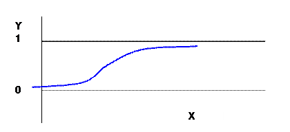
want to somehow "bend" the predicted Y-value so that the prediction of Y never goes above 1 or below zero, something like:

Probit Model

where is the cdf of the standard normal
is not constant

Logit Model

, where
is not constant

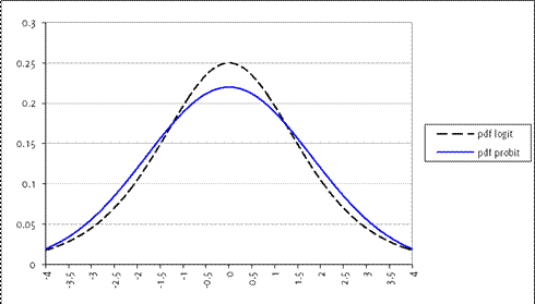
differences (Excel sheet: probit_logit_compare.xls)

Clearly the differences are rather small; it is rare that we might have a serious theoretical justification for one specification rather than the other.

(Note that the logit function given above has standard error of so in the plots I scaled the probit by this factor).

Measures of Fit

no single measure is adequate; many have been proposed
What probability should be used as "hit"? If the model says there is a 90% chance of Y=1, and it truly is equal to one, then that is reasonable to count as a correct prediction. But many measures use 50% as the cutoff. Tradeoff of false positives versus false negatives – loss function might well be asymmetric

How to do them in SPSS:

for logit: Analyze\Regression\Binary Logistic…

SPSS will generate lots of output; you can safely ignore just about everything in "Block 0" and concentrate on "Block 1". The last table shows "Variables in the equation" with columns for B, S.E., Wald, df, Sig., and Exp(B). The column for B is the estimate of the coefficient and S.E. is its standard error, same as always. But we don't estimate a t-stat but instead a Wald stat (a more complicated formula, don't worry) which combines with df to get a Sig. (a p-value). As usual, if the Sig. (p-value) is less than 0.05 then the variable is significant at the 5% level and you can make confident deductions from it. For now don't worry if you don't remember all of the details about the difference between t-tests and Wald tests from your stats classes. Just look at the calculated p-value to figure out which coefficients are significant. (Tests of multiple restrictions, which we did for the OLS model, are more complicated here so, again, don't worry about those now.)

for probit (Analyze\Regression\Probit…), SPSS wants the dependent variable (Response Frequency) and then Total Observed. For "Total Observed" just create a new variable that is always equal to 1 ("Transform\Compute" then create a new variable, ones, which always equals 1) and insert that variable. Leave "Factors" blank and insert the explanatory variables as "Covariate(s)"

SPSS calculates Probit with numerical iterations so it will sometimes return the message

Convergence Information

	Number of Iterations	Optimal Solution Found
PROBIT	20	No(a)

a Parameter estimates did not converge.

In this case, in the dialog box for "probit" usually you can choose the "Options… " button, then under "Criteria" increase the "maximum iterations" – as high as 999 if you have a small sample. The default number of iterations is just 20, which is often far too small! Sometimes, however, even 999 isn't enough. In that case, try a different program or a different set of variables. (Sometimes try the simple OLS version, which can at least catch some basic mistakes. Near-multicollinearity can kill you.)
After a successful estimation, SPSS will give you output like this:

Convergence Information

	Number of Iterations	Optimal Solution Found
PROBIT	26	Yes

The interpretation is analogous to OLS: the "Regression Coeff." is the coefficient on that variable, the "Standard Error" is its standard error, and the "Coeff./S.E." can be interpreted as a t-statistic. The remainder of the SPSS output can be safely ignored.

SPSS is generally lousy at logit/probit regressions of the type we're trying to do. It's just not designed for it. Stata is much better. If your final project involves limited dependent variables then learn Stata.
Details of estimation

recall that OLS just gives a convenient formula for finding the values of that minimize the sum . If we didn't know the formulas we could just have a computer pick values until it found the ones that made that squared term the smallest.
similarly a probit or logit coefficient estimates are finding the values of that minimize , whether the function is a normal c.d.f. or a logit c.d.f.
Maximum Likelihood (ML) is a more sophisticated way to find these coefficient estimates – better than just guessing randomly.
For example the likelihood of any particular value from a normal distribution is the p.d.f., . If we have 2 independent observations, from a distribution that is known to be normally distributed with variance of 1 (to keep the math easy) then the joint likelihood is . We want to find a value of µ that maximixes that function. This is an ugly function but we could note that any value of µ that maximizes the natural log of that function will also maximize the function itself (since is monotonic) so we take logs to get . Take the derivative with respect to µ and set it equal to zero to get so that . You should be able to see that starting with observations would get us so the average is also the maximum-likelihood estimator. A maximum-likelihood estimator could be similarly derived in cases where we don't know the variance (interestingly, that ML estimator of the standard error divides by n not (n – 1) so it is biased but consistent).
Maximizing the likelihood of the probit model is one or two steps more complicated but not different conceptually. Having a likelihood function with a first and second derivative makes finding a maximum much easier than the random hunt.

Properly Interpreting Coefficient Estimates:

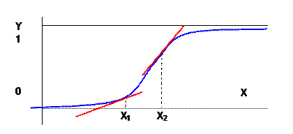
Since the slope, , the change in probability per change in X-variable, is always changing, the simple coefficients of the linear model cannot be interpreted as the slope, as we did in the OLS model. (Just like when we added a squared term, the interpretation of the slope got more complicated.)

Return to the picture to make this much clearer:

The slope at X₁ is rather low; the slope at X₂ is much steeper.

The effect of the coefficients now interacts with all of the other variables in the model: for example the effect of a person's gender on their probability of having health insurance will depend on other factors like their age and educational level. Women are generally less likely to have their own insurance than men, but how much less? Among young people with very low education, neither men nor women are very likely to be insured; among older people with very high education both are very likely insured. The biggest difference is toward the middle.

For example, very simple logit and probit estimations on the CPS 2008 dataset gives the following coefficient estimates (I am suppressing notation on significance since it is not important here):

	Logit	Probit
female	-0.428	-0.263
afam	0.220	0.134
asian	0.252	0.153
Amindian	0.012	0.007
Hispanic	-0.028	-0.015
ed_hs	0.987	0.603
ed_smcol	1.180	0.724
ed_coll	1.652	1.014
ed_adv	1.927	1.178
marrd	0.492	0.307
divwidsp	0.875	0.541
union	1.336	0.791
veteran	0.088	0.052
immig	-0.277	-0.166
imm2gen	-0.067	-0.041
Intercept	-1.303	-0.802

The probability of having health insurance varies for different socioeconomic groups. We can interpret the signs in a straightforward way: the negative coefficients on the "female" variable indicate that women are less likely to have health insurance. Surprisingly, African-Americans are more likely, along with Asians and Native Americans (although the last is not significant). Hispanics are less likely although this is also not significant.

But how large are these differences? For example, how much less likely to have health care are immigrants? It depends on the other variables. Intuitively, if a person is male, highly-educated, married, and unionized then he's probably insured (being an immigrant would them only slightly less so). So the change in probability associated with immigrant status would be low. At the opposite end, a woman without even a high school diploma, who is single, might already be unlikely to be insured. Immigrant status hardly changes this. Only in the middle will there be a big effect.

We can calculate it straightforwardly, though.

Consider, say, a non-immigrant woman with an advanced degree, whose predicted probability of having health insurance is =

Summing the 3 relevant coefficients (the intercept, female, and an advanced degree) gives a logit probability of . For an otherwise-identical immigrant woman (also with an advanced degree) the probability is 0.4796, so the change in probability is about 7%.

Comparing the probit estimates, we would just change the functional form (using the normal cdf instead of the logit function) and find a probability for a non-immigrant woman as 0.5447 and the immigrant woman to be 0.4786, with a difference of 6.6%. These estimates from the logit and probit are very close.

Compare the change in probabilities for a married male with an advanced degree who is a union member, who is either an immigrant or not. Now the probability of having insurance is, by the logit, 0.9206 for the non-immigrant and 0.8979 for the immigrant, a change of just 2.3%. From the probit the estimated probabilities are 0.9298 for the non-immigrant and 0.9045 for the immigrant, a change of 2.5%. This is because a married male with an advanced degree who is a union member is already highly likely to have health insurance, so the difference of being an immigrant or not makes only a small change compared with the previous example of a female with a high education (but unmarried and not in a union).

The details of this calculation are in an Excel spreadsheet, probit_logit_results_fromCPS2008.xls, that you can download.