Lecture Notes 2 Econ B2000, MA Econometrics Kevin R Foster, CCNY Fall 2012

 

 

Discrete Random Variables

 

For any discrete random variable, the mean or expected value is:

 

and the variance is

  so the standard deviation is the square root.

 

Can be described by PDF or CDF.  The PDF shows the probability of events; the CDF shows the cumulative probability of an event that is smaller than or equal to that event.

 

Linear Transformations:

·         If  then Y will have mean  and standard deviation .

·         If  then ;  (and if X and Y are independent then the covariance term drops out)

 

WARNING: These statements DO NOT work for non-linear calculations!  The propositions above do NOT tell about when X and Y are multiplied and divided: the distributions of  or  are not easily found.  Nor is , nor .  We might wish for a magic wand to make these work out simply but they don't in general.

 

 

Common Discrete Distributions:

Uniform

·         depend on only upper and lower bound, so all events are in

·         mean is ; standard deviation is

·         Many null hypotheses are naturally formulated as stating that some distribution is uniform: e.g. stock picks, names and grades, birth month and sports success, etc.

from: Barnett, Adrian G. (2010) The relative age effect in Australian Football League players. Working Paper.

 

Bernoulli

·         depend only on p, the probability of the event occurring

·         mean is p; standard deviation is

o   Where is max?  Intuition: what probability will give the most variation in yes/no answers?  Or use calculus; note that has same maximum as p(1 – p) so take derivative of that, set to zero

·         for coin flips, dice rolls, events with "yes/no" answers: Was person re-employed after layoff? Did patient improve after taking the drug?  Did company pay out to investors from IPO?

 

Binomial

·         have n Bernoulli trials; record how many were 1 not zero

·         ;  

o   These formulas are easy to derive from rules of linear combinations.  If B_i are independent random variables with Bernoulli distributions, then what is the mean of B₁ + B₂?  What is its std dev?

o   What if this is expressed as a fraction of trials?  Derive.

·         what fraction of coin flips came up heads?  What fraction of people were re-employed after layoff?  What fraction of patients improved?  What fraction of companies offereed IPOs?

·         questions about opinion polls – the famous "plus or minus 2 percentage points"

o   get margin of error depending on sample size (n)

o   from above, figure that mean of the fraction of people who agree or support some candidate is p, the true value, with standard error of .

 

Some students are a bit puzzled by two different sets of formulas for the binomial distribution – the standard deviation is listed as  and .  Which is it?!

 

It depends on the units.  If we measure the number of successes in n trials, then we multiply by n.  If we measure the fraction of successes in n trials, then we don't multiply but divide.

 

Consider a simple example: the probability of a hit is 50% so .   If we have 10 trials and ask, how many are likely to hit, then this should be a different number than if we had 500 trials.  The standard error of the raw number of how many, of 10, hits we would expect to see, is  which is 1.58, so with a 95% probability we would expect to see 5 hits, plus or minus 1.96*1.58 = 3.1 so a range between 2 and 8.  If we had 500 trials then the raw number we'd expect to see is 250 with a standard error or  = 11.18 so the 95% confidence interval is 250 plus or minus 22 so the range between 228 and 272.  This is a bigger range (in absolute value) but a smaller part of the fraction of hits.

 

With 10 draws, we just figured out that the range of hits is (in fractions) from 0.2 to 0.8.  With 500 draws, the range is from 0.456 to 0.544 – much narrower.  We can get these latter answers if we take the earlier result of standard deviations and divide by n.  The difference in the formula is just this result, since .  You could think of this as being analogous to the other "standard error of the average" formulas we learned, where you take the standard deviation of the original sample and divide by the square root of n.

 

Poisson

·         model arrivals per time, assuming independent

·         depends only on  which is also mean

·         PDF is

·         model how long each line at grocery store is, how cars enter traffic, how many insurance claims

 

Example of a very simple model (too simple)

 

Use computer to create models of stock price movements.  What model?  How complicated is "enough"?

 

Start really simple: Suppose the price were 100 today, and then each day thereafter it rises/falls by 10 basis points.  What is the distribution of possible stock prices, after a year (250 trading days)?

 

Use Excel (not even SPSS for now!)   First, set the initial price at 100; enter 100 into cell B2 (leaves room for labels).  Put the trading day number into column A, from 1 to 250 (shortcut).  In B1 put the label, "S".   Then label column C as "up" and in C2 type the following formula, =IF(RAND()>0.5,1,0) The "RAND()" part just picks a random number between 0 and 1 (uniformly distributed).  If this is bigger than one-half then we call it "up"; if it's smaller then we call it "down".  So that is the "=IF(statement, value-if-true, value-if-false)" portion.  So it will return a 1 if the random number is bigger than one-half and zero if not.   Then label column D as "down" and in D2 just type =1-C2 Which simply makes it zero if "up" is 1 and 1 if "up" is 0.   Then, in B3, put in the following formula, =B2*(1+0.001*(C2-D2))   Copy and paste these into the remaining cells down to 250.   Of course this isn't very realistic but it's a start.   Then plot the result (highlight columns A&B, then "Insert\Chart\XY (Scatter)"); here's one of mine:

Here are 10 series (copied and pasted the whole S, "up," and "down" 10 times), see Excel sheet "Lecturenotes2".

 

We're not done yet; we can make it better.  But the real point for now is to see the basic principle of the thing: we can simulate stock price paths as random trips.

 

The changes each day are still too regular – each day is 10 bps up or down; never constant, never bigger or smaller.  That's not a great model for the middle parts.  But the regularity within each individual series does not necessarily mean that the final prices (at step 250) are all that unrealistic.

 

I ran 2000 simulations; this is a histogram of the final price of the stock:

 

 

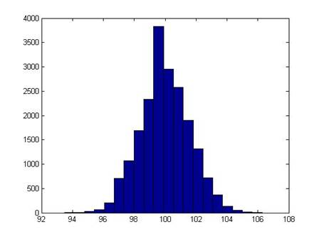
It shouldn't be a surprise that it looks rather normal (it is the result of a series of Bernoulli trials – that's what the Law of Large Numbers says should happen!).

 

With computing power being so cheap (those 2000 simulations of 250 steps took a few seconds) these sorts of models are very popular (in their more sophisticated versions).

 

It might seem more "realistic" if we thought of each of the 250 tics as being a portion of a day.  ("Realistic" is a relative term; there's a joke that economists, like artists, tend to fall in love with their models.)

 

There are times (in finance for some option pricing models) when even this very simple model can be useful, because the fixed-size jump allows us to keep track of all of the possible evolutions of the price.

 

But clearly it's important to understand Bernoulli trials summing to Binomial distributions converging to normal distributions.