|
Lecture Notes 7 Econ B2000, MA Econometrics Kevin R Foster, CCNY Fall 2012 |
|
|
Nonlinear Regression
(more properly, How to Jam Nonlinearities into a Linear Regression)
· X, X2, X3, … Xr
· ln(X), ln(Y), both ln(Y) & ln(X)
· dummy variables
· interactions of dummies
· interactions of dummy/continuous
· interactions of continuous variables
There are many examples of, and reasons for, nonlinearity. In fact we can think that the most general case is nonlinearity and a linear functional form is just a convenient simplification which is sometimes useful. But sometimes the simplification has a high price. For example, my kids believe that age and height are closely related – which is true for their sample (i.e. mostly kids of a young age, for whom there is a tight relationship, plus 2 parents who are aged and tall). If my sample were all children then that might be a decent simplification; if my sample were adults then that's lousy.
The usual justification for a linear regression is that, for any differentiable function, the Taylor Theorem delivers a linear function as being a close approximation – but this is only within a neighborhood. We need to work to get a good approximation.
Nonlinear terms
We can return to our regression using CPS data. First, we might want to ask why our regression is linear. This is mostly convenience, and we can easily add non-linear terms such as Age2, if we think that the typical age/wage profile looks like this:
So the regression would be:
(where the term "..." indicates "other stuff" that should be in the regression).
As we remember from calculus,
so that the extra “boost” in wage from another birthday might fall as the person gets older, and even turn negative if the estimate of (a bit of algebra can solve for the top of the hill by finding the Age that sets ).
We can add higher-order effects as well. Some labor econometricians argue for including Age3 and Age4 terms, which can trace out some complicated wage/age profiles. However we need to be careful of "overfitting" – adding more explanatory variables will never lower the R2.
Logarithms
Similarly can specify X or Y as ln(X) and/or ln(Y). But we've got to be careful: remember from math (or theory of insurance from Intermediate Micro) that E[ln(Y)] IS NOT EQUAL TO ln(E[Y]) ! In cases where we're regressing on wages, this means that the log of the average wage is not equal to the average log wage.
(Try it. Go ahead, I'll wait.)
When both X and Y are measured in logs then the coefficients have an easy economic interpretation. Recall from calculus that with and , so -- our usual friend, the percent change. So in a regression where both X and Y are in logarithms, then is the elasticity of Y with respect to X.
Also, if Y is in logs and D is a dummy variable, then the coefficient on the dummy variable is just the percent change when D switches from zero to one.
So the choice of whether to specify Y as levels or logs is equivalent to asking whether dummy variables are better specified as having a constant level effect (i.e. women make $10,000 less than men) or having a percent change effect (women make 25% less than men). As usual there is no general answer that one or the other is always right!
Recall our discussion of dummy variables, that take values of just 0 or 1, which we’ll represent as Di. Since, unlike the continuous variable Age, D takes just two values, it represents a shift of the constant term. So the regression,
shows that people with D=0 have intercept of just b0, while those with D=1 have intercept equal to b0 + b3. Graphically, this is:
We need not assume that the b3 term is positive – if it were negative, it would just shift the line downward. We do however assume that the rate at which age increases wages is the same for both genders – the lines are parallel.
The equation could be also written as
.
Dummy Variables Interacting with Other Explanatory Variables
The assumption about parallel lines with the same slopes can be modified by adding interaction terms: define a variable as the product of the dummy times age, so the regression is
or
or
so that, for those with D=0, as before =b1 but for those with D=1, . Graphically,
so now the intercepts and slopes are different.
So we might wonder if men and women have a similar wage-age profile. We could fit a number of possible specifications that are variations of our basic model that wage depends on age and age-squared. The first possible variation is simply that:
,
which allows the wage profile lines to have different intercept-values but otherwise to be parallel (the same hump point where wages have their maximum value), as shown by this graph:
The next variation would be to allow the lines to have different slopes as well as different intercepts:
which allows the two groups to have different-shaped wage-age profiles, as in this graph:
(The wage-age profiles might intersect or they might not – it depends on the sample data.)
We can look at this alternately, that for those with D=0,
so the extreme value of Age (where ) is .
While for those with D=1,
so the extreme value of Age (where ) is . Or write the general value, for both cases, as where D is 0 or 1.
This specification, with a dummy variable multiplying each term: the constant and all the explanatory variables, is equivalent to running two separate regressions: one for men and one for women:
Where the new coefficients are related to the old by the identities: , , and . Sometimes breaking up the regressions is easier, if there are large datasets and many interactions.
Multiple Dummy Variables
Multiple dummy variables, D1,i , D2,i , …,DJ,i, operate on the same basic principle. Of course we can then have many further interactions! Suppose we have dummies for education and immigrant status. The coefficient on education would tell us how the typical person (whether immigrant or native) fares, while the coefficient on immigrant would tell us how the typical immigrant (whatever her education) fares. An interaction of “more than Bachelor’s degree” with “Immigrant” would tell how the typical highly-educated immigrant would do beyond how the “typical immigrant” and “typical highly-educated” person would do (which might be different, for both ends of the education scale).
Many, Many Dummy Variables
Don't let the name fool you – you'd have to be a dummy not to use lots of dummy variables. For example regressions to explain people's wages might use dummy variables for the industry in which a person works. Regressions about financial data such as stock prices might include dummies for the days of the week and months of the year.
Dummies for industries are often denoted with labels like "two-digit" or "three-digit" or similar jargon. To understand this, you need to understand how the government classifies industries. A specific industry might get a 4-digit code where each digit makes a further more detailed classification. The first digit refers to the broad section of the economy, as goods pass from the first producers (farmers and miners, first digit zero) to manufacturers (1 in the first digit for non-durable manufacturers such as meat processing, 2 for durable manufacturing, 3 for higher-tech goods) to transportation, communications and utilities (4), to wholesale trade (5) then retail (6). The 7's begin with FIRE (Finance, Insurance, and Real Estate) then services in the later 7 and early 8 digits while the 9 is for governments. The second and third digits give more detail: e.g. 377 is for sawmills, 378 for plywood and engineered wood, 379 for prefabricated wood homes. Some data sets might give you 5-digit or even 6-digit information. These classifications date back to the 1930s and 1940s so some parts show their age: the ever-increasing number of computer parts go where plain "office supplies" used to be.
The CPS data distinguishes between "major industries" with 16 categories and "detailed industry" with about 50. Creating 50 dummy variables could be tiresome so I recommend that you use SPSS's syntax editor that makes cut-and-paste work easier. For example use the buttons to "compute" the first dummy variable then "Paste Syntax" to see the general form. Then copy-and-paste and change the number for the 51 variables:
COMPUTE d_ind1 = (a_dtind EQ 1).
COMPUTE d_ind2 = (a_dtind EQ 2).
COMPUTE d_ind3 = (a_dtind EQ 3).
COMPUTE d_ind4 = (a_dtind EQ 4).
COMPUTE d_ind5 = (a_dtind EQ 5).
COMPUTE d_ind6 = (a_dtind EQ 6).
COMPUTE d_ind7 = (a_dtind EQ 7).
You get the idea – take this up to 51. Then add them to your regression!
In other models such as predictions of sales, the specification might include a time trend (as discussed earlier) plus dummy variables for days of the week or months of the year, to represent the typical sales for, say, "a Monday in June".
If you're lazy like me, you might not want to do all of this mousework. (And if you really have a lot of variables, then you don't even have to be lazy.) There must be an easier way!
There is.
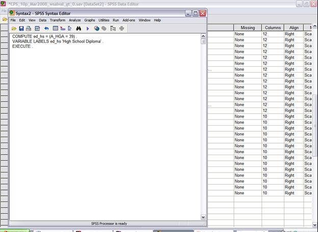
SPSS is a graphical interface that basically writes SPSS code, which is then submitted to the program. Clicking the buttons is writing computer code. Look again at this screen, where I've started coding the next dummy variable, ed_hs (from Transform\Compute Variables…)
![]()

That little button, "Paste," can be a lot of help. It pastes the SPSS code that you just created with buttons into the SPSS Syntax Editor.
Why is this helpful? Because you can copy and paste these lines of code, if you are only going to make small changes to create a bunch of new variables. So, for example, the education dummies could be created with this code:
COMPUTE ed_hs = (A_HGA = 39) .
VARIABLE LABELS ed_hs 'High School Diploma' .
COMPUTE ed_smc = (A_HGA > 39) & (A_HGA < 43) .
VARIABLE LABELS ed_smc 'Some College' .
COMPUTE ed_coll = (A_HGA = 43) .
VARIABLE LABELS ed_coll 'College 4 Year Degree' .
COMPUTE ed_adv = (A_HGA > 43) .
VARIABLE LABELS ed_adv 'Advanced Degree' .
EXECUTE .
Then choose "Run\All" from the drop-down menus to have SPSS execute the code.
You
can really see the time-saving element if, for example, you want to create
dummies for geographical area. There is
a code, GEDIV, that tells what section of the country the respondent lives
in. Again these numbers have absolutely
no inherent value, they're just codes from 1,
COMPUTE geo_1 = (GEDIV = 1) .
COMPUTE geo_2 = (GEDIV = 2) .
COMPUTE geo_3 = (GEDIV = 3) .
COMPUTE geo_4 = (GEDIV = 4) .
COMPUTE geo_5 = (GEDIV = 5) .
COMPUTE geo_6 = (GEDIV = 6) .
COMPUTE geo_7 = (GEDIV = 7) .
COMPUTE geo_8 = (GEDIV = 8) .
COMPUTE geo_9 = (GEDIV = 9) .
EXECUTE.
You can begin to realize the time-saving capability here. Later we might create 50 detailed industry and 25 detailed occupation dummies.
If at some point you get stuck (maybe the "Run" returns errors) or if you don't know the syntax to create a variable, you can go back to the button-pushing dialogue box.
The final advantage is that, if you want to do the same commands on a different dataset (say, the March 2009) then as long as you have saved the syntax you can easily submit it again.
With enough dummy variables we can start to create some respectable regressions!
Use "Data\Select Cases…" to use only those with a non-zero wage. Then do a regression of wage on Age, race & ethnicity (create some dummy variables for these), educational attainment, and geographic region.
Why am I making you do all of this? Because I want you to realize all of the choices that go into creating a regression or doing just about anything with data. There are a host of choices available to you. Some choices are rather conventional (for example, the education breakdown I used above) but you need to know the field in order to know what assumptions are common. Sometimes these commonplace assumptions conceal important information. You want to do enough experimentation to understand which of your choices are crucial to your results. Then you can begin to understand how people might analyze the exact same data but come to varying conclusions. If your results contradict someone else's, then you have to figure out what are the important assumptions that create the difference.
|
Instrumental Variables |
|
|
- Endogenous vs. Exogenous variables
- Exogenous variables are generated from "exo" outside of the model; endogenous are generated from "endo" within the model. Of course this neat binary distinction rarely is matched by the world; some variables are more endogenous than others
- Data can only demonstrate correlations – we need theory to get to causation. "Correlation does not imply causation." Roosters don't make the sun rise.
- In any regression, the variables on the right-hand side should be exogenous while the left-hand side should be endogenous, so X causes Y, . But we should always ask if it might be plausible for Y to cause X, , or for both X and Y to be caused by some external factor. If we have a circular chain of causation (so and ) then the OLS estimates are meaningless for describing causation.
- NEVER regress Price on a Quantity or vice versa!
Why never regress Price on Quantity? Wouldn't this give us a demand curve? Or would it give us a supply curve? Why would we expect to see one and not the other?
In actuality, we don't observe either supply curves or demand curves. We only observe the values of price and quantity where the two intersect.
If both vary randomly then we will not observe a supply or a demand curve. We will just observe a cloud of random points.
For example, theory says we see this:

But in the world, we assume the dotted-lines and only actually observe the one intersection, the dot:
In the next time period, supply and demand shift randomly by a bit, so theory tells us that we now have:
But again we actually now see just two points,
In the third period,
but again, in actuality just three points:
So if we tried to draw a regression line on these three points, we might convince ourselves that we had a supply curve. But do we, really? You should be able to re-draw the lines to show that we could have a down-sloping line, or a line with just about any other slope.
So even if we could wait until the end of time and see an infinite number of such points, we'd still never know anything about supply and demand. This is the problem of endogeneity. The regression is not identified – we could get more and more information but still never learn anything.
We could show this in an Excel sheet, too, which will allow a few more repetitions.
Recall that we can write a demand curve as Pd = A – BQd and a supply curve as Ps = C + DQs, where generally A, B, C, and D are all positive real numbers. In equilibrium Pd=Ps and Qd=Qs. For simplicity assume that A=10, C=0, and B=D=1. Without any randomness this would be a boring equation; solve to find 10 – Q = Q and Q*=5, P*=5. (You did this in Econ 101 when you were a baby!) If there were a bit of randomness then we could write and . Now the equilibrium conditions tell that and so and .
Plug this into Excel, assuming the two errors are normally distributed with mean zero and standard deviation of one, and find that the scatter looks like this (with 30 observations):
You can play with the spreadsheet, hit F9 to recalculate the errors, and see that there is no convergence, there is nothing to be learned.
On the other hand, what if the supply errors were smaller than the demand errors, for example by a factor of 4? Then we would see something like this:
So now with the supply curve pinned down (relatively) we can begin to see it emerge as the demand curve varies.
But note the rather odd feature: variation in demand is what identifies the supply curve; variation in supply would likewise identify the demand curve. If some of that demand error were observed then that would help identify the supply curve, or vice versa. So sometimes in agricultural data we would use weather variation (that affects the supply of a commodity) to help identify demand.
If you want to get a bit crazier, experiment if the slope terms have errors as well (so and ).
|
Notes on Measuring Discrimination – Oaxaca Decompositions: |
|
|
(much of this discussion is based on Chapter 10 of George Borjas' textbook on Labor Economics)
The regressions that we've been using measured the returns to education, age, and other factors upon the wage. If we classify people into different groups, distinguished by race, ethnicity, gender, age, or other categories, we can measure the difference in wages earned. There are many explanations but we want to determine how much is due to discrimination and how much due to different characteristics (chosen or given).
Consider a simple model where we examine the native/immigrant wage gap, and so measure , the average wages that natives get, and , the average wages that immigrants get. The simple measure, , of the wage gap, would not be adequate if natives and migrants differ in other ways, as well.
Consider the effect of age. Theory implies that people choose to migrate early in life, so we might expect to see age differences between the groups. And of course age influences the wage. If natives and immigrants had different average wages solely because of having different average ages, we would conclude very different reasons for this than if the two groups had identical ages but different wages.
For example, in a toy-sized 1000-observation subset of CPS March 2005 data, there are 406 natives and 77 immigrants workers with non-zero wages. The natives averaged wage/salary of $37,521 while the immigrants had $32,507. The average age of the natives was 39.5; the average age of the immigrants was 42.1. We want to know how much of the difference in wage can be explained by the difference in age.
Consider a simple model that posits different simple regressions for natives and immigrants:
.
We know that average wages for natives depend on average age of natives, :
and for immigrants as well, wages depend on immigrants' average age, :
.
The difference in average wages is:
but we can add and subtract the cross term, , to get:
.
Each term can be interpreted in different ways. The first difference, , is the difference in intercepts, the parallel shift of wages for all ages. The second, , is the difference in how the skills are rewarded: if everyone in the data were to have the same age, immigrants and natives would still have different wages due to these first two factors. The third is , which gives the difference in wage attributable only to differences in average age (even if those were rewarded equally). The first two are generally regarded as due to discrimination while the last is not.
The basic framework can be extended to other observable differences: in years of education, experience, or the host of other qualifications that affect people's wages and salaries.
From our discussions of regression models, we realize that the two equations above could be combined into a single framework. If we define an immigrant dummy variable as , which is equal to one if individual i is an immigrant and zero if that person is native born, we can write a regression model as:
,
where wages for natives depend on only and ,
while the immigrant coefficients are and . We
construct and so the
.
We note that unobserved differences in quality of skills can be measured as instead being due to discrimination. In our example, suppose that natives get a greater salary as they age due to the skills which they amass, but immigrants who have language difficulties learn new skills more slowly. In this case, older natives would earn more, increasing the returns to aging. This would be reflected as lower coefficients on age for immigrants than natives, and so evidence of discrimination. If we had information on English-language ability (SAT, TOEFL or GRE scores, maybe?), then the regression would show that a lack of those skills led to lower wages – no longer would it be measured as evidence of discrimination.
But this elides the question of how people gain the
"skills" measured in the first place.
If a degree from a foreign university gets less reward than a degree
from an American university, is this entirely due to discrimination? What fraction of the wage differential arises
from skill differences? In the
Consider the sort of dataset that we've been working with. Regressing Age, an Immigrant dummy, and an Age-Immigrant interaction on Wage provides the following coefficient estimates (for the same sub-sample as before):
where the immigrant dummy is actually positive (neither the immigrant dummy nor the immigrant-age interaction term are statistically significant, but I ignore that for now). With the average ages from above (natives 39.5 years old; immigrants 42.1), we calculate the gap in average predicted wages (natives are predicted to make an average wage of $37,561; immigrants to make $32,502) is $5058.08. The two first terms in the Oaxaca decomposition, relating to unexplained factors such as "discrimination" account for $5329.95, while the difference in age accounts for just -$271.86 (a negative amount) – this means that the ages actually imply that natives and immigrants ought to be closer in wages so they are even farther apart. We might reasonably believe that much of this difference reflects omitted factors (and could list out the important omitted factors); this is intended merely as an exercise.
Adding these additional variables is easy; I show the case for two variables but the model can be extended to as many variables as are of interest. Next consider a more complicated model, where now wages depend on Age and Education, so the two regressions for natives and immigrants are:
.
We know that average wages for natives depend on average age and education of natives, :
and for immigrants as well, wages depend on immigrants' average age, :
.
The difference in average wages is:
but we can add and subtract the cross terms , to get:
.
Again, the two terms showing the difference in average levels of external factors, and , are "explained" by the model while the other terms showing the difference in the coefficients are "unexplained" and could be considered as evidence of discrimination.
Exercises:
- Do the above analysis on the current CPS data.
- If instead you used log wages, but still kept just age as the measured variable, is your answer substantially different than in the previous question? (Note that the answers are in different units, so you have to think about how to convert the two answers.)
- Consider
other measures of skills, such as schooling and whatever other factors you
consider important. How does this
new regression change the
- What is the maximum fraction of wage difference that you can find (with different independent variables and regression specifications), related to discrimination? The minimum?
References:
Borjas, George (2003). Labor Economics.