|
Practice for Exam 1 Econ B2000, MA Econometrics Kevin R Foster, CCNY Fall 2012 |
|
|
Not all of these questions are strictly relevant; some might require a bit of knowledge that we haven't covered this year, but they're a generally good guide.
1. (15 points) You might find it useful to sketch the distributions.
a. For a Standard Normal Distribution, what is the area closer to the mean than 1.45?
b. For a Standard Normal Distribution, what is the area to the right of 2?
c. For a Normal Distribution with mean 5 and standard deviation 7.6, what is area to the right of 14.1?
d. For a Normal Distribution with mean 1 and standard deviation 7.8, what is area in both tails farther from the mean than 11?
e. For a Normal Distribution with mean -5 and standard deviation 1.6, what is area in both tails farther from the mean than -2.6?
f. For a Normal Distribution with mean -1 and standard deviation 9.8, what values leave probability 0.157 in both tails?
2. (15 points) In a medical study (reference below), people were randomly assigned to use either antibacterial products or regular soap. In total 592 people used antibacterial soap; 586 used regular soap. It was found that 33.1% of people using antibacterial products got a cold; 32.3% of people using regular soap got colds.
a. Test the null hypothesis that there is no difference in the rates of sickness for people using regular or antibacterial soap. (What is the p-value?)
b. Create a 95% confidence interval for the difference in sickness rates. What is the 90% confidence interval? The 99% interval?
c. Every other study has found similar results. Why do you think people would pay more for antibacterial soaps?
E.L.Larson, S.X. Lin, C. Gomez-Pichardo, P. Della-Latta, (2004). "Effect of Antibacterial Home Cleaning and Handwashing Products on Infectious Disease Symptoms: A Randomized Double-Blind Trial," Ann Intern Med, 140(5), 321-329.
3. (15 points) A study of workers and managers asked both how much management listened to workers' suggestions (on a scale of 1-7 where "1" indicates that they paid great attention). Managers averaged a 2.50 (standard deviation of 0.55); workers answered an average 2.08 (standard deviation of 0.76) – managers ignore their workers even more often than the employees realize. There were 137 workers and 14 managers answering.
a. Test the null hypothesis that there was no difference between workers and managers: how likely is it that there is actually no difference in average response? (What is the p-value?)
b. Create a 95% confidence interval for the difference between workers and managers. What is the 90% confidence interval? The 99% interval?
4. (15 points) A recent survey by Intel showed that 53% of parents (561 were surveyed) were uncomfortable talking with their children about math & science. Previous surveys found that 57% of parents talked with their kids about sex & drugs.
a. Test the null hypothesis that parents are as comfortable talking about math & science as sex & drugs; that the true value of parents uncomfortable with math and science is not different from 57%. What is the p-value?
b. Create a 95% confidence interval for the true fraction of parents who are uncomfortable with math & science. What is the 90% confidence interval? The 99% interval?
5. (15 points) The New York Times reported on educational companies that over-sell their products and gave the example of "Cognitive Tutor" (CT) that helps math students. The CT students improved by 17.41 (standard error of 5.82); the regular students improved by 15.28 (standard error of 5.33). There were 153 students in the new program and 102 regular students.
a. Test the null hypothesis that there is no difference between regular students and those in the CT group. What is the p-value for this difference?
b. Create a 95% confidence interval for the difference between regular and CT students. What is the 90% confidence interval? The 99% interval?
6. (20 points) Use the ATUS data (available from Blackboard) on the time that people spend in different activities.
a. Among households with kids, what is the average time spent on activities related to kids?
b. Among households with kids, how much time to men and women spend on activities related to kids? Form a hypothesis test for whether there is a statistically significant difference between the time that men and women spend with kids. What is the p-value for the hypothesis of no difference? What is a 95% confidence interval for the difference in time?
c. Why do you think that we would find these results? Explain (perhaps with some further empirical results from the same data set).
7. (25 points) Use the PUMS data (available from Blackboard) on the residents of NYC. Consider the time (in minutes) spent by people to travel to work; this variable has name JWMNP.
a. How many men and women answered this question? What variables do you think would be relevant, in trying to explain the variation in commuting times?
b. Form a linear regression with the dependent variable, "JWMNP Travel Time to Work," and relevant independent variables.
c. Which independent variables have coefficients that are statistically significantly different from zero?
8. {{this question was given in advance for students to prepare with their group} Download (from Blackboard) and prepare the dataset on the 2004 Survey of Consumer Finances from the Federal Reserve. Estimate the probability that each head of household (restrict to only heads of household!) has at least one credit card. Write up a report that explains your results (you might compare different specifications, you might consider different sets of socioeconomic variables, different interactions, different polynomials, different sets of fixed effects, etc.).
9. Explain in greater detail your topic for the final project. Include details about the dataset which you will use and the regressions that you will estimate. Cite at least one previous study which has been done on that topic (published in a refereed journal).
10. This question refers to your final project.
a. What data set will you use?
b. What regression (or regressions) will you run? Explain carefully whether the dependent variable is continuous or a dummy, and what this means for the regression specification. What independent variables will you include?
c. What other variables are important, but are not measured and available in your data set? How do these affect your analysis?
11. You want to examine the impact of higher crude oil prices on American driving habits during the past oil price spike. A regression of US gasoline purchases on the price of crude oil as well as oil futures gives the coefficients below. Critique the regression and explain whether the necessary basic assumptions hold. Interpret each coefficient; explain its meaning and significance.
Coefficients(a)
|
Model |
|
Unstandardized Coefficients |
Standardized Coefficients |
t |
Sig. |
|
| B |
Std. Error |
Beta |
||||
|
1 |
(Constant) |
.252 |
.167 |
|
1.507 |
.134 |
| return on crude futures, 1 month ahead |
.961 |
.099 |
.961 |
9.706 |
.000 |
|
| return on crude futures, 2 months ahead |
-.172 |
.369 |
-.159 |
-.466 |
.642 |
|
| return on crude futures, 3 months ahead |
.578 |
.668 |
.509 |
.864 |
.389 |
|
| return on crude futures, 4 months ahead |
-.397 |
.403 |
-.333 |
-.986 |
.326 |
|
| US gasoline consumption |
-.178 |
.117 |
-.036 |
-1.515 |
.132 |
|
| Spot Price Crude Oil Cushing, OK WTI FOB (Dollars per Barrel) |
4.23E-005 |
.000 |
.042 |
1.771 |
.079 |
|
a Dependent Variable: return on crude spot price
12. You are in charge of polling for a political campaign. You have commissioned a poll of 300 likely voters. Since voters are divided into three distinct geographical groups, the poll is subdivided into three groups with 100 people each. The poll results are as follows:
|
|
|
total |
|
A |
B |
C |
|
|
number in favor of candidate |
170 |
|
58 |
57 |
55 |
|
|
number total |
300 |
|
100 |
100 |
100 |
|
|
std. dev. of poll |
0.4956 |
|
0.4936 |
0.4951 |
0.4975 |
Note that the standard deviation of the sample (not the standard error of the average) is given.
d. Calculate a t-statistic, p-value, and a confidence interval for the main poll (with all of the people) and for each of the sub-groups.
e. In simple language (less than 150 words), explain what the poll means and how much confidence the campaign can put in the numbers.
f. Again in simple language (less than 150 words), answer the opposing candidate's complaint, "The biased media confidently says that I'll lose even though they admit that they can't be sure about any of the subgroups! That's neither fair nor accurate!"
13. Fill in the blanks in the following table showing SPSS regression output. The model has the dependent variable as time spent working at main job.
Coefficients(a)
|
Model |
|
Unstandardized Coefficients |
Standardized Coefficients |
t |
Sig. |
|
| B |
Std. Error |
Beta |
||||
|
1 |
(Constant) |
198.987 |
7.556 |
|
26.336 |
.000 |
| female |
-65.559 |
4.031 |
-.138 |
___?___ |
___?___ |
|
| African-American |
-9.190 |
6.190 |
-.013 |
___?___ |
___?___ |
|
| Hispanic |
17.283 |
6.387 |
.024 |
___?___ |
___?___ |
|
| Asian |
1.157 |
12.137 |
.001 |
___?___ |
___?___ |
|
| Native American/Alaskan Native |
-28.354 |
14.018 |
-.017 |
-2.023 |
.043 |
|
| Education: High School Diploma |
___?___ |
6.296 |
.140 |
11.706 |
.000 |
|
| Education: Some College |
___?___ |
6.308 |
.174 |
14.651 |
.000 |
|
| Education: 4-year College Degree |
110.064 |
___?___ |
.183 |
16.015 |
.000 |
|
| Education: Advanced degree |
126.543 |
___?___ |
.166 |
15.714 |
.000 |
|
| Age |
-1.907 |
___?___ |
-.142 |
-16.428 |
.000 |
|
a Dependent Variable: Time Working at main job
14. Suppose I were to start a hedge fund, called KevinNeedsMoney Limited Ventures, and I want to present evidence about how my fund did in the past. I have data on my fund's returns, Rett, at each time period t, and the returns on the market, Mktt. The graph below shows the relationship of these two variables:
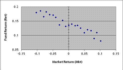
a. I run a univariate OLS regression, . Approximately what value would be estimated for the intercept term, b0? For the slope term, b1?
b. How would you describe this fund's performance, in non-technical language – for instance if you were advising a retail investor without much finance background?
15. Using the American Time Use Study (ATUS) we measure the amount of time that each person reported that they slept. We run a regression to attempt to determine the important factors, particularly to understand whether richer people sleep more (is sleep a normal or inferior good) and how sleep is affected by labor force participation. The SPSS output is below.
|
Coefficients(a) |
|
|
|
|
|
||
|
Model
|
Unstandardized Coefficients |
Standardized Coefficients |
|
|
|||
|
|
|
B |
Std. Error |
Beta |
t |
Sig. |
|
|
1 |
(Constant) |
-4.0717 |
4.6121 |
|
-0.883 |
0.377 |
|
|
|
female |
23.6886 |
1.1551 |
0.18233 |
20.508 |
0.000 |
|
|
|
African-American |
-8.5701 |
1.7136 |
-0.04369 |
-5.001 |
0.000 |
|
|
|
Hispanic |
10.1015 |
1.7763 |
0.05132 |
5.687 |
0.000 |
|
|
|
Asian |
-1.9768 |
3.3509 |
-0.00510 |
-0.590 |
0.555 |
|
|
|
Native American/Alaskan Native |
-3.5777 |
3.8695 |
-0.00792 |
-0.925 |
0.355 |
|
|
|
Education: High School Diploma |
2.5587 |
1.8529 |
0.01768 |
1.381 |
0.167 |
|
|
|
Education: Some College |
-0.3234 |
1.8760 |
-0.00222 |
-0.172 |
0.863 |
|
|
|
Education: 4-year College Degree |
-1.3564 |
2.0997 |
-0.00821 |
-0.646 |
0.518 |
|
|
|
Education: Advanced degree |
-3.3303 |
2.4595 |
-0.01590 |
-1.354 |
0.176 |
|
|
|
Weekly Earnings |
0.000003 |
0.000012 |
-0.00277 |
-0.246 |
0.806 |
|
|
|
Number of children under 18 |
2.0776 |
0.5317 |
0.03803 |
3.907 |
0.000 |
|
|
|
person is in the labor force |
-11.6706 |
1.7120 |
-0.08401 |
-6.817 |
0.000 |
|
|
|
has multiple jobs |
0.4750 |
2.2325 |
0.00185 |
0.213 |
0.832 |
|
|
|
works part time |
4.2267 |
1.8135 |
0.02244 |
2.331 |
0.020 |
|
|
|
in school |
-5.4641 |
2.2993 |
-0.02509 |
-2.376 |
0.017 |
|
|
|
Age |
1.1549 |
0.1974 |
0.31468 |
5.850 |
0.000 |
|
|
|
Age-squared |
-0.0123 |
0.0020 |
-0.33073 |
-6.181 |
0.000 |
|
a. Which variables are statistically significant at the 5% level? At the 1% level?
b. Are there other variables that you think are important and should be included in the regression? What are they, and why?
16. Use the SPSS dataset, atus_tv from Blackboard, which is a subset of the American Time Use survey. This time we want to find out which factors are important in explaining whether people spend time watching TV. There are a wide number of possible factors that influence this choice.
a. What fraction of the sample spend any time watching TV? Can you find sub-groups that are significantly different?
b. Estimate a regression model that incorporates the important factors that influence TV viewing. Incorporate at least one non-linear or interaction term. Show the SPSS output. Explain which variables are significant (if any). Give a short explanation of the important results.
17. Estimate the following regression:: S&P100 returns = b0 + b1(lag S&P100 returns) + b2(lag interest rates) + ε
using the dataset, financials.sav. Explain which coefficients (if any) are significant and interpret them.
18. A study by Mehran and Tracy examined the relationship between stock option grants and measures of the company's performance. They estimated the following specification:
Options = b0+b1(Return on Assets)+b2(Employment)+b3(Assets)+b4(Loss)+u
where the variable (Loss) is a dummy variable for whether the firm had negative profits. They estimated the following coefficients:
|
|
Coefficient |
Standard Error |
|
Return on Assets |
-34.4 |
4.7 |
|
Employment |
3.3 |
15.5 |
|
Assets |
343.1 |
221.8 |
|
Loss Dummy |
24.2 |
5.0 |
Which estimate has the highest t-statistic (in absolute value)? Which has the lowest p-value? Show your calculations. How would you explain the estimate on the "Loss" dummy variable?
19. Calculate the probability in the following areas under the Normal pdf with mean and standard deviation as given. You might usefully draw pictures as well as making the calculations. For the calculations you can use either a computer or a table.
g. What is the probability, if the true distribution has mean -15 and standard deviation of 9.7, of seeing a deviation as large (in absolute value) as -1?
h. What is the probability, if the true distribution has mean 0.35 and standard deviation of 0.16, of seeing a deviation as large (in absolute value) as 0.51?
i. What is the probability, if the true distribution has mean -0.1 and standard deviation of 0.04, of seeing a deviation as large (in absolute value) as -0.16?
20. Using data from the NHIS, we find the fraction of children who are female, who are Hispanic, and who are African-American, for two separate groups: those with and those without health insurance. Compute tests of whether the differences in the means are significant; explain what the tests tell us. (Note that the numbers in parentheses are the standard deviations.)
|
|
with health insurance |
without health insurance |
|
female |
0.4905 (0.49994) N=7865 |
0.4811 (0.49990) N=950 |
|
Hispanic |
0.2587 (0.43797) N=7865 |
0.5411 (0.49857) N=950 |
|
African American |
0.1785 (0.38297) N=7865 |
0.1516 (0.35880) N=950 |
21. A paper by Farber examined the choices of how many hours a taxidriver would work, depending on a number of variables. His output is:
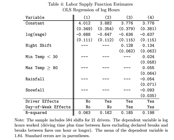
"Driver Effects" are fixed effects for the 21 different drivers.
a. What is the estimated elasticity of hours with respect to the wage?
b. Is there a significant change in hours on rainy days? On snowy days?
22. For the ATUS dataset, use "Analyze \ Descriptive Statistics \ Crosstabs" to create a joint probability table showing the fractions of males/females about the amount of time spent on the computer vs watching TV (if either or both are above average). Find and interpret the joint probabilities and marginal probabilities. Do this for age groups as well.
23. Calculate the probability in the following areas under the Standard Normal pdf with mean of zero and standard deviation of one. You might usefully draw pictures as well as making the calculations. For the calculations you can use either a computer or a table.
a. What is the probability, if the true distribution is a Standard Normal, of seeing a deviation from zero as large (in absolute value) as 1.9?
b. What is the probability, if the true distribution is a Standard Normal, of seeing a deviation from zero as large (in absolute value) as -1.5?
c. What is the probability, if the true distribution is a Standard Normal, of seeing a deviation as large (in abs0lute value) as 1.2?
24. Calculate the probability in the following areas under the Normal pdf with mean and standard deviation as given. You might usefully draw pictures as well as making the calculations. For the calculations you can use either a computer or a table.
a. What is the probability, if the true distribution has mean -1 and standard deviation of 1.5, of seeing a deviation as large (in absolute value) as 2?
b. What is the probability, if the true distribution has mean 50 and standard deviation of 30, of seeing a deviation as large (in absolute value) as 95?
c. What is the probability, if the true distribution has mean 0.5 and standard deviation of 0.3, of seeing a deviation as large (in absolute value) as zero?
25. A paper by Chiappori, Levitt, and Groseclose (2002) looked at the strategies of penalty kickers and goalies in soccer. Because of the speed of the play, the kicker and goalie must make their decisions simultaneously (a Nash equilibrium in mixed strategies). For example, if the goalie moves to the left when the kick also goes to the left, the kick scores 63.2% of the time; if the goalie goes left while the kick goes right, then the kick scores 89.5% of the time. In the sample there were 117 occurrences when both players went to the left and 95 when the goalie went left while the kick went right. What is the p-value for a test that the probability of scoring is different? What advice, if any, would you give to kickers, based on these results? Why or why not?
26. A paper by Claudia Goldin and Cecelia Rouse (1997) discusses the fraction of men and women who are hired by major orchestras after auditions. Some orchestras had applicants perform from behind a screen (so that the gender of the applicant was unknown) while other orchestras did not use a screen and so were able to see the gender of the applicant. Their data show that, of 445 women who auditioned from behind a screen, a fraction 0.027 were "hired". Of the 599 women who auditioned without a screen, 0.017 were hired. Assume that these are Bernoulli random variables. Is there a statistically significant difference between the two samples? What is the p-value? Explain the possible significance of this study.
27. Another paper, by Kristin Butcher and Anne Piehl (1998), compared the rates of institutionalization (in jail, prison, or mental hospitals) among immigrants and natives. In 1990, 7.54% of the institutionalized population (or 20,933 in the sample) were immigrants. The standard error of the fraction of institutionalized immigrants is 0.18. What is a 95% confidence interval for the fraction of the entire population who are immigrants? If you know that 10.63% of the general population at the time are immigrants, what conclusions can be made? Explain.
28. Calculate the probability in the following areas under the Standard Normal pdf with mean of zero and standard deviation of one. You might usefully draw pictures as well as making the calculations. For the calculations you can use either a computer or a table.
a. What is the probability, if the true distribution is a Standard Normal, if seeing a value as large as 1.75?
b. What is the probability, if the true distribution is a Standard Normal, if seeing a value as large as 2?
c. If you observe a value of 1.3, what is the probability of observing such an extreme value, if the true distribution were Standard Normal ?
d. If you observe a value of 2.1, what is the probability of observing such an extreme value, if the true distribution were Standard Normal ?
e. What are the bounds within which 80% of the probability mass of the Standard Normal lies?
f. What are the bounds within which 90% of the probability mass of the Standard Normal lies?
g. What are the bounds within which 95% of the probability mass of the Standard Normal lies?
29. Consider a standard normal pdf with mean of zero and standard deviation of one.
a. Find the area under the standard normal pdf between -1.75 and 0.
b. Find the area under the standard normal pdf between 0 and 1.75.
c. What is the probability of finding a value as large (in absolute value) as 1.75 or larger, if it truly has a standard normal distribution?
d. What values form a symmetric 90% confidence interval for the standard normal (where symmetric means that the two tails have equal probability)? A 95% confidence interval?
30. Now consider a normal pdf with mean of 3 and standard deviation of 4.
a. Find the area under the normal pdf between 3 and 7.
b. Find the area under the normal pdf between 7 and 11.
c. What is the probability of finding a value as far away from the mean as 7 if it truly has a normal distribution?
31. If a random variable is distributed normally with mean 2 and standard deviation of 3, what is the probability of finding a value as far from the mean as 6.5?
32. If a random variable is distributed normally with mean -2 and standard deviation of 4, what is the probability of finding a value as far from the mean as 0?
33. If a random variable is distributed normally with mean 2 and standard deviation of 3, what values form a symmetric 90% confidence interval?
34. If a random variable is distributed normally with mean 2 and standard deviation of 2, what is a symmetric 95% confidence interval? What is a symmetric 99% confidence interval?
35. A random variable is distributed as a standard normal. (You are encouraged to sketch the PDF in each case.)
a. What is the probability that we could observe a value as far or farther than 1.7?
b. What is the probability that we could observe a value nearer than 0.7?
c. What is the probability that we could observe a value as far or farther than 1.6?
d. What is the probability that we could observe a value nearer than 1.2?
e. What value would leave 15% of the probability in the left tail?
f. What value would leave 10% of the probability in the left tail?
36. A random variable is distributed with mean of 8 and standard deviation of 4. (You are encouraged to sketch the PDF in each case.)
a. What is the probability that we could observe a value lower than 6?
b. What is the probability that we could observe a value higher than 12?
c. What is the probability that we'd observe a value between 6.5 and 7.5?
d. What is the probability that we'd observe a value between 5.5 and 6.5?
e. What is the probability that the standardized value lies between 0.5 and -0.5?
37. You know that a random variable has a normal distribution with standard deviation of 16. After 10 draws, the average is -12.
a. What is the standard error of the average estimate?
b. If the true mean were -11, what is the probability that we could observe a value between -10.5 and -11.5?
38. You know that a random variable has a normal distribution with standard deviation of 25. After 10 draws, the average is -10.
a. What is the standard error of the average estimate?
b. If the true mean were -10, what is the probability that we could observe a value between -10.5 and -9.5?
39. You are consulting for a polling organization. They want to know how many people they need to sample, when predicting the results of the gubernatorial election.
a. If there were 100 people polled, and the candidates each had 50% of the vote, what is the standard error of the poll?
b. If there were 200 people polled?
c. If there were 400 people polled?
d. If one candidate were ahead with 60% of the vote, what is the standard error of the poll?
e. They want the poll to be 95% accurate within plus or minus 3 percentage points. How many people do they need to sample?
40. Using the ATUS dataset that we've been using in class, form a comparison of the mean amount of TV time watched by two groups of people (you can define your own groups, based on any of race, ethnicity, gender, age, education, income, or other of your choice).
a. What are the means for each group? What is the average difference?
b. What is the standard deviation of each mean? What is the standard error of each mean?
c. What is a 95% confidence interval for each mean?
d. Is the difference statistically significant?
Exam 1
41. (15 points) Calculate the probability in the following areas under the Standard Normal pdf with mean of zero and standard deviation of one. You might usefully draw pictures as well as making the calculations. For the calculations you can use either a computer or a table.
d. What is the probability, if the true distribution is a Standard Normal, of seeing a deviation from zero as large (in absolute value) as 1.9?
e. What is the probability, if the true distribution is a Standard Normal, of seeing a deviation from zero as large (in absolute value) as -1.5?
f. What is the probability, if the true distribution is a Standard Normal, of seeing a deviation as large (in abs0lute value) as 1.2?
42. (15 points) Calculate the probability in the following areas under the Normal pdf with mean and standard deviation as given. You might usefully draw pictures as well as making the calculations. For the calculations you can use either a computer or a table.
d. What is the probability, if the true distribution has mean -1 and standard deviation of 1.5, of seeing a deviation as large (in absolute value) as 2?
e. What is the probability, if the true distribution has mean 50 and standard deviation of 30, of seeing a deviation as large (in absolute value) as 95?
f. What is the probability, if the true distribution has mean 0.5 and standard deviation of 0.3, of seeing a deviation as large (in absolute value) as zero?
43. (20 points) Below is some SPSS output from a regression from the ATUS. The data encompass only the group of people who report that they spent non-zero time in education-related activities such as going to class or doing homework for class. The regression examines the degree to which education-time crowds out TV-watching time. The dependent is time spent watching TV. The independents are time spent on all Education-related activities as well as the usual demographic variables. Fill in the blanks.
Coefficients(a)
|
Model |
|
Unstandardized Coefficients |
Standardized Coefficients |
t |
Sig. |
|
| B |
Std. Error |
Beta |
||||
|
1 |
(Constant) |
160.531 |
14.658 |
|
10.952 |
.000 |
| time spent on Education-related activities |
-.137 |
.023 |
-.224 |
__?__ |
__?__ |
|
| female |
-26.604 |
7.852 |
-.112 |
__?__ |
__?__ |
|
| African-American |
-4.498 |
__?__ |
-.014 |
-.417 |
.677 |
|
| Hispanic |
__?__ |
12.181 |
-.023 |
-.681 |
.496 |
|
| Asian |
-7.881 |
19.291 |
-.013 |
__?__ |
__?__ |
|
| Native American/Alaskan Native |
-4.335 |
28.633 |
-.005 |
-.151 |
__?__ |
|
| Education: High School Diploma |
1.461 |
13.415 |
.004 |
.109 |
__?__ |
|
| Education: Some College |
3.186 |
__?__ |
.012 |
.311 |
.756 |
|
| Education: 4-year College Degree |
-47.769 |
13.471 |
-.144 |
-3.546 |
__?__ |
|
| Education: Advanced degree |
__?__ |
18.212 |
-.131 |
-3.379 |
.001 |
|
| Age |
__?__ |
.276 |
.121 |
2.839 |
.005 |
|
| Weekly earnings [2 implied decimals] |
.000 |
.000 |
-.041 |
-.990 |
.322 |
|
| In the Labor Force |
-25.210 |
10.794 |
-.107 |
__?__ |
.020 |
|
| Has multiple jobs |
.918 |
15.299 |
.002 |
__?__ |
.952 |
|
| Works part time |
3.816 |
10.427 |
.015 |
.366 |
.714 |
|
a Dependent Variable: watching TV (not religious)
44. Using the same SPSS output from the regression above, explain clearly which variables are statistically significant. Provide an interpretation for each of the observed signs. What about the magnitude of the coefficients? What additional variables (that are in the dataset) should be included? What results are surprising to you? (Note your answer should be a well-written few paragraphs, not just terse answers to the above questions.)
45. Use the CPS dataset (available from Blackboard) to do a regression. Explain why your dependent variable might be caused by your independent variable(s). What additional variables (that are in the dataset) might be included? Why did you exclude those? Next examine the regression coefficients. Which ones are significant? Do the signs match what would be predicted by theory? Are the magnitudes reasonable? (Note your answer should be a well-written few paragraphs, not just terse answers to the above questions. No SPSS output dumps either!)
46. A colleague proposes the following fitted line. Explain how or if his model could be an OLS regression. There are 100 observations of pairs of and for simplicity assume for all . For the first 99 observations, the fitted value, , is equal to the actual value, so . But for the 100th observation the fitted value misses the true value by 2, so . If the fitted values do not come from an OLS regression, how should the fitted model be changed?