Class Nov 14
Kevin R Foster, CCNY, ECO B2000
Fall 2013
Experiments and Quasi-Experiments
- ideal: double-blind random sort into treatment and base sets
- differences estimator
- Problems can be internal:
- incomplete randomization
- failure to follow treatment protocol
- attrition
- experiment
(
- or external
- non-representative sample
- non-rep program
- treatment/eligibility
- general equilibrium effects
Time Series
Basic definitions:
- first difference VYt = Yt – Yt-1
- percent change is
 and is
approximately equal to ln(Yt)
– ln(Yt-1) – this log approximation is commonly
used
and is
approximately equal to ln(Yt)
– ln(Yt-1) – this log approximation is commonly
used - lags: the first lag of Yt is Yt-1; second lag is Yt-2, etc.
- Autocorrelation: how
strong is last period data related to this period? The autocorrelation coefficient is
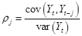 for each lag
length, j. Sometimes plot a graph
of the autocorrelation coefficients for various j.
for each lag
length, j. Sometimes plot a graph
of the autocorrelation coefficients for various j. - Common assumption: Stationarity: a model that explains Y doesn't change over time – the future is like the past, so there's some point to examining the past – a crucial assumption in forecasting! But this is why we usually use stock returns not stock price – the price is not likely stationary even if returns are. (Also often assume ergodic.)
- If autocorrelations are not zero, then OLS is not appropriate estimator if X and Y are both time series! The standard errors are a function of the autocorrelation terms so cannot properly evaluate the regression.
- Seasonality is
basically a regression with seasons (months, days, whatever) as dummy
variables. So could have
 - remember to
leave one dummy variable out! Or
- remember to
leave one dummy variable out! Or  .
.
Types of Models
- AR(1) – autoregression with lag 1
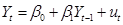
- Forecast error is one-step-ahead error
- Note that can re-write
the AR(1) equation, by substituting
 , as
, as  , then substitute in for
 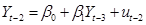 , and so on. So
the current value is a function of all past error terms,
, and so on. So
the current value is a function of all past error terms,
 . Note that as
long as
. Note that as
long as  , the last term drops and the sums converge as
  .
. - Reminder of convergent
series: look at
 , note that
  . Add and
subtract
. Add and
subtract  and fiddle the
parentheses to write
and fiddle the
parentheses to write  . Notate that
ugly term
. Notate that
ugly term  , then the equation says that
  . Solve,
  , and
, and  . Substitute this
into the previous equation for Yt
. Substitute this
into the previous equation for Yt 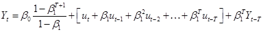 . As , the first term goes to
  , the last term goes to zero, and the middle term is
  .
.- If
 then none of the
terms converge – the model becomes a random walk or integrated with order
1, I(1) or has a unit root. (Can test for this, most common is
Augmented Dickey-Fuller ADF.)
then none of the
terms converge – the model becomes a random walk or integrated with order
1, I(1) or has a unit root. (Can test for this, most common is
Augmented Dickey-Fuller ADF.) - Also
random walk with trend, so
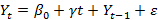
- And
random walk with drift, so
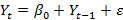 (but no trend)
 - Or just plain random walk,

- Random walk means that AR coefficients are biased toward zero, the t-statistics (and therefore p-values) are unreliable, and we can have a "spurious regression" – two time series that seem related only because both increase over time
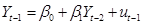
- AR(p) – autoregression with lag p

- ADL(p,q) – autoregressive distributed lag model with p lags of dependent variable and q lags of an additional predictor, X.
- Need usual assumptions for this model
- Lag length? Some art; some science! Various criteria (AIC, BIC, given in text) to select lag length.
- Granger Causality – jargon meaning that X helps predict Y; more precisely X does not Granger-cause Y if X does not help predict Y. If X does not help predict Y then it cannot cause Y.
- Trends provide non-stationary models
- Random walk non-stationary model:
- Breaks can also give non-stationary models
- test for breaks, sup-Wald test
- Can model time series as regression of Y on X, of ln(Y) on ln(X), of DY on DX, or of %DY on %DX (where, recall, %DY = DlnY since the derivative of the log is the reciprocal) – this is where the art comes in!
- Distributed lag models can be complicated (Chapter 15) and so we want at a minimum Heteroskedasticy and Autocorrelation Consistent (HAC) errors – like the heteroskedasticity-consistent errors before (Newey-West)
- VAR – Vector AutoRegression, incorporate k regressors and p lags so estimate as many as k*p coefficients – these are classic in macro modeling, following work of Chris Sims
- GARCH models – Generalized AutoRegressive Conditional Heteroskedasticity models – allow the variance of the error to change over time, depending on past errors – allows "storms" of volatility followed by quiet (low-variance)
 GARCH(p,q)
- Combine with random walk analysis for IGARCH, etc
In R: read “Time Series Analysis with R” for a high-level overview of what’s possible – that has refs to various packages that you can study, as you figure out what exactly you want to do. http://www.stats.uwo.ca/faculty/aim/tsar/
Non-Parametric Regression
Instead of assuming a functional form – that the age-wage profile is linear, or quadratic, or cubic, or whatever … just let the data determine the wiggles in the function.
Details in R program.
Factor Analysis
Another common procedure, particularly in finance, is a factor analysis. This asks whether a variety of different variables can be well explained by common factors. Sometimes when it's not clear about the direction of causality, or where the modeler does not want to impose an assumption of causality, this can be a way to express how much variation is common. As an example. one price that people often see, which changes very often, is the price of gasoline. If you have data on the prices at different gas stations over a long period of time, you would basically see that while the prices are not identical, they move together over time. This is not surprising since the price of oil fluctuates. There might be interesting variation that at some times certain stations might be more or less responsive to price changes – but overall the story would be that there is a common influence.
Factor Analysis (and the related technique of Principal Components Analysis, PCA) are not model-based and can be useful methods of exploration. An example might be the easiest way to see how it works.
I have data from the US Energy Information Administration (EIA) on the spot and futures prices of gasoline from 2005-2012. (Spot prices are the price paid for delivery today; futures prices are prices agreed now for delivery in a few months.) The prices also differ depending on where they were delivered since the price of gasoline varies over different parts of the country – although we usually only hear about it when something goes wrong with the system (e.g. a refinery must be closed or a storm damages a port or pipeline) and the variation becomes large. We would have every reason to expect that these prices ought to be highly correlated. With SPSS we can use "Analyze \ Dimension Reduction \ Factor". This gives us output like this:
|
Total Variance
Explained |
||||||
|
Component |
Initial Eigenvalues |
Extraction Sums of
Squared Loadings |
||||
|
Total |
% of Variance |
Cumulative % |
Total |
% of Variance |
Cumulative % |
|
|
1 |
5.908 |
98.470 |
98.470 |
5.908 |
98.470 |
98.470 |
|
2 |
.057 |
.952 |
99.422 |
|
|
|
|
3 |
.019 |
.320 |
99.742 |
|
|
|
|
4 |
.010 |
.172 |
99.914 |
|
|
|
|
5 |
.003 |
.055 |
99.969 |
|
|
|
|
6 |
.002 |
.031 |
100.000 |
|
|
|
|
Extraction Method: Principal Component
Analysis. |
||||||
If you've taken linear algebra you'll recognize the eigenvalue as determining the common variation. In this case, looking at the third column, "% of Variance," we see that the first component explains 98.470% of the variation in the 6 variables. The additional factors (up to 6) make little additional contribution. So in this case it is reasonable to represent these 6 price series as being mostly (more than 98%) explained by a single common factor.
So from the output,
|
Component Matrixa |
|
|
|
Component |
|
1 |
|
|
Futures1Month |
.996 |
|
Futures2Months |
.997 |
|
Futures3Months |
.995 |
|
Futures4Months |
.989 |
|
NYGasSpot |
.993 |
|
GulfGasSpot |
.985 |
|
Extraction Method: Principal Component
Analysis. |
|
|
a. 1 components extracted. |
|
This gives the "loading" of the factor on each of the variables, which is the correlation of the factor with the variable. In this case it is difficult to perceive much difference.
For another example, consider daily data on US interest rates at various maturities (from the Federal Reserve website). The maturities are the Fed Funds (overnight), 4 weeks, 3 and 6 months, 1 year Treasuries, and swap rates at 1, 2, 3, 4, 5, 7, 10, and 30 years. The output shows,
|
Total Variance Explained |
||||||
|
Component |
Initial Eigenvalues |
Extraction Sums of Squared Loadings |
||||
|
Total |
% of Variance |
Cumulative % |
Total |
% of Variance |
Cumulative % |
|
|
1 |
11.035 |
84.882 |
84.882 |
11.035 |
84.882 |
84.882 |
|
2 |
1.406 |
10.816 |
95.698 |
1.406 |
10.816 |
95.698 |
|
3 |
.448 |
3.450 |
99.148 |
|
|
|
|
4 |
.058 |
.444 |
99.592 |
|
|
|
|
5 |
.031 |
.235 |
99.827 |
|
|
|
|
6 |
.011 |
.086 |
99.912 |
|
|
|
|
7 |
.006 |
.046 |
99.958 |
|
|
|
|
8 |
.004 |
.028 |
99.986 |
|
|
|
|
9 |
.001 |
.009 |
99.996 |
|
|
|
|
10 |
.000 |
.003 |
99.999 |
|
|
|
|
11 |
.000 |
.001 |
100.000 |
|
|
|
|
12 |
2.848E-05 |
.000 |
100.000 |
|
|
|
|
13 |
1.895E-05 |
.000 |
100.000 |
|
|
|
|
Extraction Method: Principal Component
Analysis. |
||||||
We see that two principal components explain over 95% of the variation.
The initial component correlation is
|
Component Matrixa |
||
|
|
Component |
|
|
1 |
2 |
|
|
Federal funds effective rate |
.903 |
-.369 |
|
3-month Treasury bill secondary market
rate discount basis |
.906 |
-.369 |
|
6-month Treasury bill secondary market
rate discount basis |
.944 |
-.317 |
|
4-week Treasury bill secondary market
rate discount basis |
.867 |
-.393 |
|
1-year Treasury bill secondary market
rate^ discount basis |
.966 |
-.242 |
|
Rate paid by fixed-rate payer on an
interest rate swap with maturity of one year. |
.913 |
-.240 |
|
Rate paid by fixed-rate payer on an
interest rate swap with maturity of two year. |
.972 |
-.041 |
|
Rate paid by fixed-rate payer on an
interest rate swap with maturity of three year. |
.975 |
.129 |
|
Rate paid by fixed-rate payer on an
interest rate swap with maturity of four year. |
.961 |
.239 |
|
Rate paid by fixed-rate payer on an
interest rate swap with maturity of five year. |
.945 |
.314 |
|
Rate paid by fixed-rate payer on an
interest rate swap with maturity of seven year. |
.917 |
.397 |
|
Rate paid by fixed-rate payer on an
interest rate swap with maturity of ten year. |
.886 |
.450 |
|
Rate paid by fixed-rate payer on an
interest rate swap with maturity of thirty year. |
.807 |
.477 |
|
Extraction Method: Principal Component
Analysis. |
||
|
a. 2 components extracted. |
||
Which is a bit difficult to interpret. We can ask SPSS to rotate the factors (click the button for "Rotation" and check "Varimax" which is the most common). For those remembering some linear algebra, this is an orthogonal rotation. The point of rotation is to help interpret the factors. A rotated factor loading is:
|
Rotated Component Matrixa |
||
|
|
Component |
|
|
1 |
2 |
|
|
Federal funds effective rate |
.912 |
.347 |
|
3-month Treasury bill secondary market
rate discount basis |
.914 |
.350 |
|
6-month Treasury bill secondary market
rate discount basis |
.906 |
.414 |
|
4-week Treasury bill secondary market
rate discount basis |
.902 |
.305 |
|
1-year Treasury bill secondary market
rate^ discount basis |
.870 |
.483 |
|
Rate paid by fixed-rate payer on an
interest rate swap with maturity of one year. |
.831 |
.449 |
|
Rate paid by fixed-rate payer on an interest
rate swap with maturity of two year. |
.738 |
.634 |
|
Rate paid by fixed-rate payer on an
interest rate swap with maturity of three year. |
.624 |
.760 |
|
Rate paid by fixed-rate payer on an
interest rate swap with maturity of four year. |
.538 |
.831 |
|
Rate paid by fixed-rate payer on an
interest rate swap with maturity of five year. |
.475 |
.875 |
|
Rate paid by fixed-rate payer on an
interest rate swap with maturity of seven year. |
.398 |
.916 |
|
Rate paid by fixed-rate payer on an
interest rate swap with maturity of ten year. |
.340 |
.934 |
|
Rate paid by fixed-rate payer on an
interest rate swap with maturity of thirty year. |
.263 |
.900 |
|
Extraction Method: Principal Component
Analysis. Rotation Method: Varimax
with Kaiser Normalization. |
||
|
a. Rotation converged in 3 iterations. |
||
Where we can clearly see that the first component is a short-term innovation with effects that die off over longer maturities while the second component is a long-term innovation with small effects on short rates but larger effects on long-term rates. This interpretation is convenient and helps us understand how interest rates in the US move. If one were hedging interest rate risk, there are a wide variety of instruments but two main components so a firm could hedge 95% of its exposure with two securities.
Econometrics goes on and on – there are thousands of techniques for new situations and new conditions, especially now that computing power quickly increases the amount of calculations that can be done. There is so much to learn!