Lecture 2: Discrete and
Continuous Random Variables
Kevin R
Foster, CCNY, ECO B2000
Fall 2013
For any discrete
random variable, the mean or expected value is:
![]()
and the variance is
![]() so
the standard deviation is the square root.
so
the standard deviation is the square root.
These can be
described by PDF or CDF – probability density function or cumulative
distribution function. The PDF shows the
probability of events; the CDF shows the cumulative probability of an event
that is smaller than or equal to that event.
The PDF is the derivative of the CDF.
Linear
Transformations:
·
If ![]() then Y will have mean
then Y will have mean ![]() and standard deviation
and standard deviation ![]() .
.
·
If ![]() then
then ![]() ;
; ![]() (and if X and Y are
independent then the covariance term drops out)
(and if X and Y are
independent then the covariance term drops out)
WARNING: These
statements DO NOT work for non-linear calculations! The propositions above do NOT tell about when
X and Y are multiplied and divided: the distributions of ![]() or
or ![]() are not easily
found. Nor is
are not easily
found. Nor is ![]() , nor
, nor ![]() . We might wish for a
magic wand to make these work out simply but they don't in general.
. We might wish for a
magic wand to make these work out simply but they don't in general.
Common
Discrete Distributions:
Uniform
·
depend on only upper and lower bound, so all
events are in ![]()
·
mean is ![]() ; standard deviation is
; standard deviation is 
·
Many null hypotheses are naturally formulated as
stating that some distribution is uniform: e.g. stock picks, names and grades,
birth month and sports success, etc.
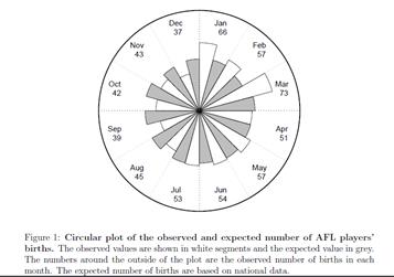
from: Barnett, Adrian G. (2010) The relative age effect in
Australian Football League players. Working Paper.
Although note
that distribution of births is not quite uniform; certainly among animal
species humans are unusual in that births are not overwhelmingly seasonal.
Benford's Law: not really a law but an empirical result
about measurements, that looking at the first digit, the value 1 is much more
common than 9 – the first digit is not uniformly distributed. Originally stated for tables of
logarithms. Second digit is closer to
uniform; third digit closer still, etc.
See online Excel sheet. This is a
warning that sometimes our intuition about how we might think numbers are
distributed is actually wrong.
Question: Does the "shuffle"
function on your music player distribute songs uniformly?
Bernoulli
·
depend only on p, the probability of the event
occurring
·
mean is p; standard deviation is ![]()
o
Where is
the maximum standard deviation?
Intuition: what probability will give the most variation in yes/no
answers? Or use calculus; note that has
same maximum as p(1 – p) so take derivative of that,
set to zero. Then hit your forehead with
the palm of your hand, realizing that calculus gave you the same answer as
simple intution.
·
Used for coin flips, dice rolls, events with
"yes/no" answers: Was person re-employed after layoff? Did patient
improve after taking the drug? Did
company pay out to investors from IPO?
Binomial
·
have n Bernoulli trials; record how many were 1
not zero
·
![]() ;
; ![]()
o
These formulas are easy to derive from rules of
linear combinations. If Bi
are independent random variables with Bernoulli distributions, then what is the
mean of B1 + B2?
What is its std dev?
o
What if this is expressed as a fraction of
trials? Derive.
·
what fraction of coin
flips came up heads? What fraction of
people were re-employed after layoff? What fraction of
patients improved? What fraction of companies offereed IPOs?
·
questions about opinion polls – the famous
"plus or minus 2 percentage points"
o
get margin of error depending on sample size (n)
o
from above, figure that
mean of the fraction of people who agree or support some candidate is p, the
true value, with standard error of ![]() .
.
Some students are a bit puzzled by two
different sets of formulas for the binomial distribution – the standard deviation
is listed as ![]() and
and ![]() . Which is it?!
. Which is it?!
It depends on the units. If we measure the number of successes in n
trials, then we multiply by n. If we measure the fraction of successes in n
trials, then we don't multiply but divide.
Consider a simple example: the
probability of a hit is 50% so ![]() . If we have 10
trials and ask, how many are likely to hit, then this should be a different
number than if we had 500 trials. The
standard error of the raw number of how many, of 10, hits we would expect to
see, is
. If we have 10
trials and ask, how many are likely to hit, then this should be a different
number than if we had 500 trials. The
standard error of the raw number of how many, of 10, hits we would expect to
see, is ![]() which is 1.58, so with
a 95% probability we would expect to see 5 hits, plus or minus 1.96*1.58 = 3.1
so a range between 2 and 8. If we had
500 trials then the raw number we'd expect to see is 250 with a standard error
or
which is 1.58, so with
a 95% probability we would expect to see 5 hits, plus or minus 1.96*1.58 = 3.1
so a range between 2 and 8. If we had
500 trials then the raw number we'd expect to see is 250 with a standard error
or ![]() = 11.18 so the 95% confidence interval is 250 plus or minus
22 so the range between 228 and 272.
This is a bigger range (in absolute value) but a smaller part of the
fraction of hits.
= 11.18 so the 95% confidence interval is 250 plus or minus
22 so the range between 228 and 272.
This is a bigger range (in absolute value) but a smaller part of the
fraction of hits.
With 10 draws, we just figured out
that the range of hits is (in fractions) from 0.2 to 0.8. With 500 draws, the range is from 0.456 to
0.544 – much narrower. We can get these latter
answers if we take the earlier result of standard deviations and divide by
n. The difference in the formula is just
this result, since ![]() . You could think of
this as being analogous to the other "standard error of the average"
formulas we learned, where you take the standard deviation of the original
sample and divide by the square root of n.
. You could think of
this as being analogous to the other "standard error of the average"
formulas we learned, where you take the standard deviation of the original
sample and divide by the square root of n.
Poisson
·
model arrivals per time, assuming independent
·
depends only on ![]() which is also mean
which is also mean
·
PDF is ![]()
·
model how long each line at grocery store is, how
cars enter traffic, how many insurance claims
From
Discrete to Continuous: an example of a very simple model (too simple)
Use computer to
create models of stock price movements.
What model? How complicated is
"enough"?
Start really
simple: Suppose the price were 100 today, and then each day thereafter it
rises/falls by 10 basis points. What is
the distribution of possible stock prices, after a year (250 trading days)?
Use Excel
(not even SPSS for now!)
|
First, set the initial price at 100;
enter 100 into cell B2 (leaves room for labels). Put the trading day number into column A,
from 1 to 250 (shortcut). In B1 put
the label, "S". Then label column C as "up"
and in C2 type the following formula, =IF( The "RAND()"
part just picks a random number between 0 and 1 (uniformly distributed). If this is bigger than one-half then we
call it "up"; if it's smaller then we call it "down". So that is the "=IF(statement,
value-if-true, value-if-false)" portion.
So it will return a 1 if the random number is bigger than one-half and
zero if not. Then label column D as
"down" and in D2 just type =1-C2 Which simply makes it zero if
"up" is 1 and 1 if "up" is 0. Then, in B3, put in the following
formula, =B2*(1+0.001*(C2-D2)) Copy and paste these into the
remaining cells down to 250. Of course this isn't very realistic
but it's a start. Then plot the result (highlight
columns A&B, then "Insert\Chart\XY (Scatter)"); here's one of
mine:
|
|
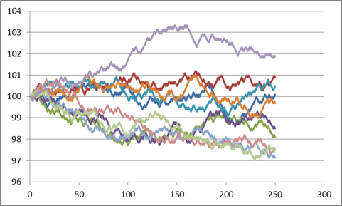
Here are 10 series (copied and pasted
the whole S, "up," and "down" 10 times), see Excel sheet
"Lecturenotes2".
|
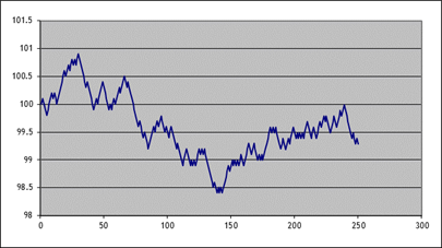
We're not done
yet; we can make it better. But the real
point for now is to see the basic principle of the thing: we can simulate stock
price paths as random trips.
The changes each
day are still too regular – each day is 10 bps up or down; never constant,
never bigger or smaller. That's not a great
model for the middle parts. But the
regularity within each individual series does not necessarily mean that the
final prices (at step 250) are all that unrealistic.
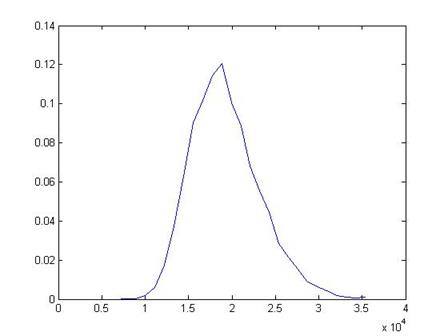
I ran 2000
simulations; this is a histogram of the final price of the stock:
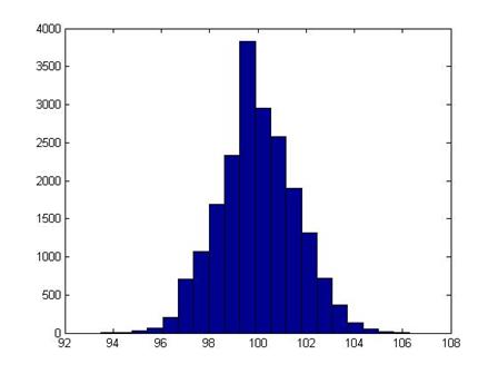
It shouldn't be a
surprise that it looks rather normal (it is the result of a series of Bernoulli
trials – that's what the Law of Large Numbers says should happen!).
With computing
power being so cheap (those 2000 simulations of 250 steps took a few seconds) these
sorts of models are very popular (in their more sophisticated versions).
It might seem
more "realistic" if we thought of each of the 250 tics as being a
portion of a day. ("Realistic"
is a relative term; there's a joke that economists, like artists, tend to fall
in love with their models.)
There are times
(in finance for some option pricing models) when even this very simple model
can be useful, because the fixed-size jump allows us to keep track of all of
the possible evolutions of the price.
But clearly it's
important to understand Bernoulli trials summing to Binomial distributions
converging to normal distributions.
Continuous
Random Variables
The PDF
and CDF
Where discrete
random variables would sum up probabilities for the individual outcomes, continuous
random variables necessitate some more complicated math. When X is a continuous random variable, the
probability of it being equal to any particular value is zero If X is continuous, there is a zero chance
that it will be, say, 5 – it could be 4.99998 or 5.000001 and so on. But we can still take the area under the PDF
by taking the limit of the sum, as the horizontal increments get smaller and
smaller – the Riemann method, for those who remember Calculus. So to find the probability of X being equal
to a set of values we integrate the PDF between those values, so
![]() .
.
The CDF, the
probability of observing a value less than some parameter, is therefore the
integral with ![]() as the lower limit of
integration, so
as the lower limit of
integration, so ![]() .
.
For this class
you aren't required to use calculus but it's helpful to see why somebody might
want to use it. (Note that many of the
statistical distributions we'll talk about come up in solving partial
differential equations such as are commonly used in finance – so if you're
thinking of a career in that direction, you'll want even more math!)
Normal
Distribution
We will most
often use the Normal Distribution – but usually the first question from
students is "Why is that crazy thing normal?!!" You're not the only one to ask
In statistics it
is often convenient to use a normal distribution, the bell-shaped distribution
that arises in many circumstances. It is
useful because the (properly scaled) mean of independent random draws of many
other statistical distributions will tend toward a normal distribution – this
is the Central Limit Theorem.
Some basic facts
and notation: a normal distribution with mean µ and standard deviation s
is denoted N(µ,s). (The variance is the square of the standard
deviation, s2.) The Standard Normal distribution is when µ=0
and s=1;
its probability density function (pdf) is denoted pdfN(x);
the cumulative density function (CDF) is cdfN(x)
or sometimes Nor(x).
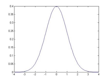
This is a graph of the PDF (the height at any point) and CDF of the
normal:

Example of using normal distributions:
A paper by
Hansen, Sato, & Ruedy (2012) showed these decadal
distributions of temperature anomalies:
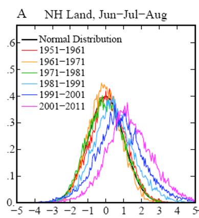
This shows the
rightward spread of temperature deviations.
The x-axis is in standard deviations, which makes the various
geographies easily comparable (a hot day in Alaska is different from a hot day
in Oklahoma). The authors define extreme
heat as more than 3 standard deviations above the mean and note that the probability
of extreme heat days has risen from less than 1% to above 10%.
One of the basic
properties of the normal distribution is that, if X is distributed normally
with mean µ and standard deviation s,
then Y = A + bX is also distributed normally, with mean
(A + bµ) and standard deviation bs. We will use this particularly when we
"standardize" a sample: by subtracting its mean and dividing by its
standard deviation, the result should be distributed with mean zero and
standard deviation 1.
Oppositely, if we
are creating random variables with a standard deviation, we can take random
numbers with a N(0,1) distribution, multiply by the
desired standard deviation, and add the desired mean, to get normal random
numbers with any mean or standard deviation.
In Excel, you can create normally distributed random numbers by using
the RAND() function to generate
uniform random numbers on [0,1], then NORMSINV(
Motivation:
Sample Averages are Normally Distributed
Before we do a
long section on how to find areas under the normal distribution, I want to
address the big question: Why we the heck would anybody ever want to know
those?!?!
Consider a case
where we have a population of people and we sample just a few to calculate an
average. Before elections we hear about
these types of procedures all of the time: a poll that samples just 1000 people
is used to give information about how a population of millions of people will
vote. These polls are usually given with
a margin of error ("54% of people liked Candidate A over B, with a margin
of error of plus or minus 2 percentage points"). If you don't know statistics then polls
probably seem like magic. If you do know
statistics then polls are based on a few simple formulas.
I have a dataset
of about 206,639 people who reported their wage and salary to a particular
government survey, the "Current Population Survey," the CPS. The true average of their wage and salaries
was $19,362.62. (Not quite; the top income value is cut at $625,000 –
people who made more are still just coded with that amount. But don't worry about that for now.) The standard deviation of the full 206,639
people is 39,971.91.
A histogram of
the data shows that most people report zero (zero is the median value), which
is reasonable since many of them are children or retired people. However some report incomes up to $625,000!
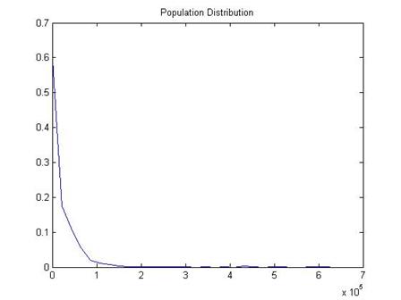
Taking an average
of a population with such extreme values would seem to be difficult.
Suppose that I
didn't want to calculate an average for all 206,639 people – I'm lazy or I've
got a real old and slow computer or whatever.
I want to randomly choose just 100 people and calculate the sample
average. Would that be "good
enough"?
Of course the
first question is "good enough for what?" – what
are we planning to do with the information?
But we can still
ask whether the answer will be very close to the true value. In this case we know the true value; in most
cases we won't. But this allows us to
take a look at how the sampling works.
Here is a plot of
values for 1000 different polls (each poll with just 100 people).
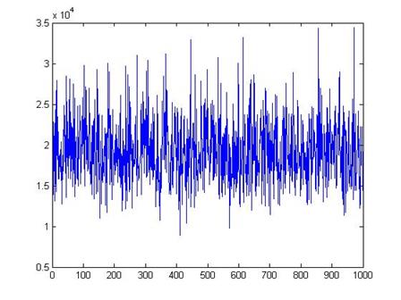
We can see that,
although there are a few polls with averages as low almost 10,000 and a few
with averages as high as 30,000, most of the polls are close to the true mean
of $19,363.
In general the
average of even a small sample is a good estimate of the true average value of
the population. While a sample might
pick up some extreme values from one side, it is also likely to pick extreme
values from the other side, which will tend to balance out.
A histogram of
the 1000 poll means is here:
This shows that
the distribution of the sample means looks like a Normal distribution – another
case of how "normal" and ordinary the Normal distribution is.
Of course the
size of each sample, the number of people in each poll, is also important. Sampling more people gets us better estimates
of the true mean.
This graph shows
the results from 100 polls, each with different sample sizes.
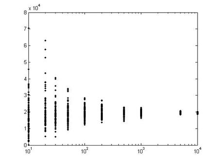
In the first set
of 100 polls, on the left, each poll has just 10 people in it, so the results
are quite varied. The next set has 20
people in each poll, so the results are closer to the true mean. By the time we get to 100 people in each poll
(102 on the log-scale x-axis), the variation in the polls is much
smaller.
Each distribution
has a bell shape, but we have to figure out if there is a single invariant
distribution or only a family of related bell-shaped curves.
If we subtract
the mean, then we can center the distribution around
zero, with positive and negative values indicating distance from the
center. But that still leaves us with
different scalings: as the graph above shows, the
typical distance from the center gets smaller.
So we divide by its standard deviation and we get a "Standard
Normal" distribution.
The Standard
Normal graph is:
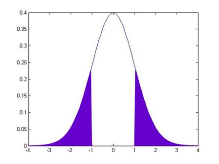
Note that it is
symmetric around zero. Like any
histogram, the area beneath the curve is a measure of the probability. The total area under the curve is exactly 1
(probabilities must add up to 100%). We
can use the known function to calculate that the area under the curve, from -1
to 1, is 68.2689%. This means that just
over 68% of the time, I will draw a value from within 1 standard deviation of
the center. The area of the curve from
-2 to 2 is 95.44997%, so we'll be within 2 standard deviations over 95.45% of
the time.
It is important
to be able to calculate areas under the Standard Normal. For this reason people used to use big tables
(statistics textbooks still have them); now we use computers. But even the computers don't always quite
give us the answer that we want, we have to be a bit savvy.
So the normal CDF
of, say, -1, is the area under the pdf of the points to the left of -1:
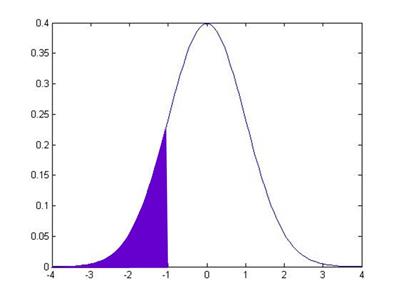
This area is
15.87%. How can I use this information
to get the value that I earlier told you, that the area in between -1 and 1 is
68.2689%? Well, we know two other things
(more precisely, I know them and I wrote them just 3 paragraphs up, so you
ought to know them). We know that the
total area under the pdf is 100%. And we
know that the pdf is symmetric around zero.
This symmetry means that the area under the other tail, the area from +1
all the way to the right, is also 15.87%.
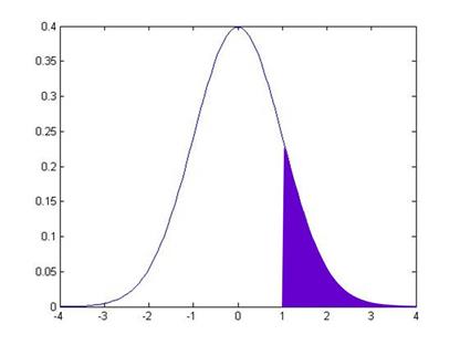
So to find the
area in between -1 and +1, I take 100% and subtract off the two tail areas:
And this middle
area is 100 – 15.87 – 15.87 = 68.26.
Sidebar: you can
think of all of this as "adding up" without calculus. On the other hand, calculus makes this procedure
much easier and we can precisely define the cdf as
the integral, from negative infinity to some point Z, under the pdf: ![]() .
.
So with just this
simple knowledge, you can calculate all sorts of areas using just the
information in the CDF.
Hints on
using Excel, SPSS, and Matlab to calculate the Standard Normal
cdf
Excel
Excel has both normdist and normsdist. For normdist, you need to tell it the mean and standard deviation, so use
the function normdist(X,mean,stdev,cumulative). For normsdist it assumes the
mean is zero and standard deviation is one so you just use normsdist(X). Read the help files to learn
more. The final argument of the normdist function,
"Cumulative" is a true/false: if true then it
calculates the cdf (area to the left of X); if false
it calculates the pdf. [Personally, that's an ugly and non-intuitive bit of coding, but then
again, Microsoft has no sense of beauty.]
To figure out the
other way – what X value gives me some particular probability, we use norminv or normsinv.
All of these
commands are under "Insert"
then "Function"
then, under "Select a Category" choose "Statistical".
Google
Mistress Google
knows all. When I google "Normal cdf calculator" I get a link to http://www.uvm.edu/~dhowell/StatPages/More_Stuff/normalcdf.html.
This is a simple and easy interface: put in the z-value to get the probability
area or the inverse. Even ask Siri!
SPSS
For SPSS you can
open it up with an empty dataset and go to the "Data View" tab.
Then use "Transform,"
"Compute Variable…"
and, under "Function Group"
find "CDF and Noncentral
CDF". Then "Cdf.Normal(X,mean,stdev)"
calculates the normal cdf for the given X
variable. Select this function and use
the up-arrow to push it into the "Numeric
Expression" dialog box. For
any of the inputs (which SPSS denotes as "?")
you can click on a variable from the list on the left. Or just type in the values. You need to give your output variable a name,
this is the blank "Target Variable"
on the upper left-hand side. If you're
just doing calculations then give it any name; later on, if you are doing more
complex series of calculations, you can worry about understandable variable
names. Then hit "OK" and look back in the "Data View." (It will spawn an Output view but that only
tells you if there were errors in the function.)
To go backwards,
find "Inverse DF"
under "Function Group"
and then "IDF.Normal(p,mean,stdev)" where you input the
probability.
Matlab
Matlab has the command,
normcdf(X,mean,stdev). The inputs mean
and stdev
are the mean and standard deviations of the normal distribution considered; for
the Standard Normal you can just leave those blank and just write normcdf(X).
If X is a vector or matrix then it computes the standard normal cdf of each cell value.
The function normpdf(X,mean,stdev)
is the pdf naturally.
Norminv(p,mean,stdev) gives the inverse of the normcdf function and normsinv(p) gives the inverse for the standard normal.
Side Note: The basic property, that the distribution is normal whatever the time
interval, is what makes the normal distribution {and related functions, called Lévy distributions} special. Most distributions would not have this
property so daily changes could have different distributions than weekly,
monthly, quarterly, yearly, or whatever!
Recall from
calculus the idea that some functions are not differentiable in places – they
take a turn that is so sharp that, if we were to approximate the slope of the
function coming at it from right or left, we would get very different answers. The function, ![]() , is an example: at zero the left-hand derivative is -1; the
right-hand derivative is 1. It is not
differentiable at zero – it turns so sharply that it cannot be well
approximated by local values. But it is
continuous – it can be continuous even if it is not differentiable.
, is an example: at zero the left-hand derivative is -1; the
right-hand derivative is 1. It is not
differentiable at zero – it turns so sharply that it cannot be well
approximated by local values. But it is
continuous – it can be continuous even if it is not differentiable.
Now suppose I had
a function that was everywhere continuous but nowhere differentiable – at every
point it turns so sharply as to be unpredictable given past values. Various such functions have been derived by
mathematicians, who call it a Wiener process (it generates Brownian
motion). (When Einstein visited CCNY in
1905 he discussed his paper using Brownian motion to explain the movements of
tiny particles in water, that are randomly bumped around by water
molecules.) This function has many
interesting properties – including an important link with the Normal
distribution. The Normal distribution
gives just the right degree of variation to allow continuity – other
distributions would not be continuous or would have infinite variance.
Note also that a
Wiener process has geometric form that is independent of scale or orientation –
a Wiener process showing each day in the year cannot be distinguished from a
Wiener process showing each minute in another time frame. As we noted above, price changes for any time
interval are normal, whether the interval is minutely, daily, yearly, or
whatever. These are fractals, curious
beasts described by mathematicians such as Mandelbrot, because normal variables
added together are still normal. (You
can read Mandelbrot's 1963 paper in the Journal of Business, which you can
download from JStor – he argues that Wiener processes
are unrealistic for modeling financial returns and proposes further
generalizations.)
The Normal
distribution has a
pdf which looks ugly but isn't so bad once you break it down. It is proportional to ![]() . This is what gives
it a bell shape:
. This is what gives
it a bell shape:
To make this a
real probability we need to have all of its area sum up to one, so the
probability density function (PDF) for a standard normal (with zero mean and
standard deviation of one) is
![]() .
.
To allow a mean,
µ, different from zero and a standard deviation, σ, different from one, we
modify the formula to this:
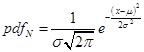 .
.
The connection
with e is useful if it reminds you of
when you learned about "natural logarithms" and probably thought
"what the heck is 'natural' about that ugly thing?!" But you learn that it comes up everywhere
(think it's bad now? wait for differential equations!) and eventually make your
peace with it. So too the 'normal'
distribution.
If you think that
the PDF is ugly then don't feel bad – its discoverer didn't like it
either. Stigler's History of Statistics
relates that Laplace first derived the function as the limit of a binomial
distribution as ![]() but couldn't believe
that anything so ugly could be true. So
he put it away into a drawer until later when Gauss derived the same formula
(from a different exercise) – which is why the Normal distribution is often
referred to as "Gaussian". The
Normal distribution arises in all sorts of other cases: solutions to partial
differential equations; in physics Maxwell used it to describe the diffusion of
gases or heat (again Brownian motion); in information theory where it is
connected to standard measures of entropy (Kullback Liebler); even in the distribution of prime factors in
number theory, the Erdős–Kac
Theorem.
but couldn't believe
that anything so ugly could be true. So
he put it away into a drawer until later when Gauss derived the same formula
(from a different exercise) – which is why the Normal distribution is often
referred to as "Gaussian". The
Normal distribution arises in all sorts of other cases: solutions to partial
differential equations; in physics Maxwell used it to describe the diffusion of
gases or heat (again Brownian motion); in information theory where it is
connected to standard measures of entropy (Kullback Liebler); even in the distribution of prime factors in
number theory, the Erdős–Kac
Theorem.
Finally I'll note
the statistical quincunx, which is a great word since it sounds naughty but is
actually geeky (google it or I'll try to get an online version to play in
class).