Class Sept 19
Kevin R Foster, CCNY, ECO B2000
Fall 2013
From Discrete to Continuous: an example of a very simple model (too simple)
Use computer to create models of stock price movements. What model? How complicated is "enough"?
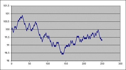
Start really simple: Suppose the price were 100 today, and then each day thereafter it rises/falls by 10 basis points. What is the distribution of possible stock prices, after a year (250 trading days)?
Use Excel (not even SPSS for now!)
|
First, set the initial price at 100;
enter 100 into cell B2 (leaves room for labels). Put the trading day number into column A,
from 1 to 250 (shortcut). In B1 put
the label, "S". Then label column C as "up"
and in C2 type the following formula, =IF( The "RAND()"
part just picks a random number between 0 and 1 (uniformly distributed). If this is bigger than one-half then we
call it "up"; if it's smaller then we call it
"down". So that is the
"=IF(statement, value-if-true,
value-if-false)" portion. So it
will return a 1 if the random number is bigger than one-half and zero if not. Then label column D as
"down" and in D2 just type =1-C2 Which simply makes it zero if
"up" is 1 and 1 if "up" is 0. Then, in B3, put in the following
formula, =B2*(1+0.001*(C2-D2)) Copy and paste these into the
remaining cells down to 250. Of course this isn't very realistic
but it's a start. Then plot the result (highlight
columns A&B, then "Insert\Chart\XY (Scatter)"); here's one of
mine:
|
|
Here are 10 series (copied and pasted
the whole S, "up," and "down" 10 times), see Excel sheet
"Lecturenotes2".
|
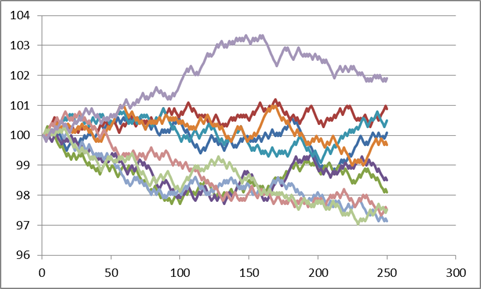
We're not done yet; we can make it better. But the real point for now is to see the basic principle of the thing: we can simulate stock price paths as random trips.
The changes each day are still too regular – each day is 10 bps up or down; never constant, never bigger or smaller. That's not a great model for the middle parts. But the regularity within each individual series does not necessarily mean that the final prices (at step 250) are all that unrealistic.
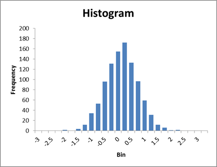
I ran 2000 simulations; this is a histogram of the final price of the stock:
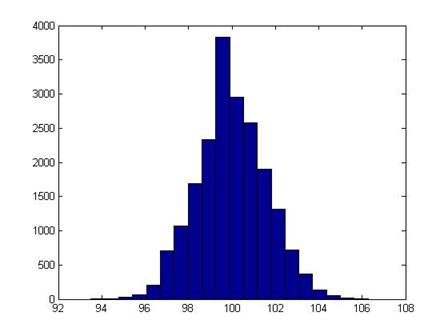
It shouldn't be a surprise that it looks rather normal (it is the result of a series of Bernoulli trials – that's what the Law of Large Numbers says should happen!).
With computing power being so cheap (those 2000 simulations of 250 steps took a few seconds) these sorts of models are very popular (in their more sophisticated versions).
It might seem more "realistic" if we thought of each of the 250 tics as being a portion of a day. ("Realistic" is a relative term; there's a joke that economists, like artists, tend to fall in love with their models.)
There are times (in finance for some option pricing models) when even this very simple model can be useful, because the fixed-size jump allows us to keep track of all of the possible evolutions of the price.
But clearly it's important to understand Bernoulli trials summing to Binomial distributions converging to normal distributions.
Continuous Random Variables
The PDF and CDF
Where discrete random variables would sum up probabilities for the individual outcomes, continuous random variables necessitate some more complicated math. When X is a continuous random variable, the probability of it being equal to any particular value is zero If X is continuous, there is a zero chance that it will be, say, 5 – it could be 4.99998 or 5.000001 and so on. But we can still take the area under the PDF by taking the limit of the sum, as the horizontal increments get smaller and smaller – the Riemann method, for those who remember Calculus. So to find the probability of X being equal to a set of values we integrate the PDF between those values, so
![]() .
.
The CDF, the
probability of observing a value less than some parameter, is therefore the
integral with ![]() as the lower limit of
integration, so
as the lower limit of
integration, so ![]() .
.
For this class you aren't required to use calculus but it's helpful to see why somebody might want to use it. (Note that many of the statistical distributions we'll talk about come up in solving partial differential equations such as are commonly used in finance – so if you're thinking of a career in that direction, you'll want even more math!)
Normal Distribution
We will most often use the Normal Distribution – but usually the first question from students is "Why is that crazy thing normal?!!" You're not the only one to ask
In statistics it is often convenient to use a normal distribution, the bell-shaped distribution that arises in many circumstances. It is useful because the (properly scaled) mean of independent random draws of many other statistical distributions will tend toward a normal distribution – this is the Central Limit Theorem.
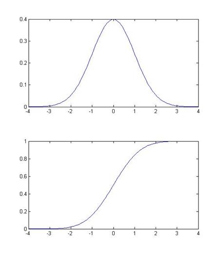
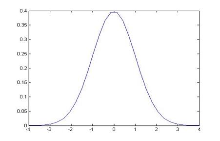
Some basic facts and notation: a normal distribution with mean µ and standard deviation s is denoted N(µ,s). (The variance is the square of the standard deviation, s2.) The Standard Normal distribution is when µ=0 and s=1; its probability density function (pdf) is denoted pdfN(x); the cumulative density function (CDF) is cdfN(x) or sometimes Nor(x). This is a graph of the PDF (the height at any point) and CDF of the normal:
Example of using normal distributions:
A paper by Hansen, Sato, & Ruedy (2012) showed these decadal distributions of temperature anomalies:
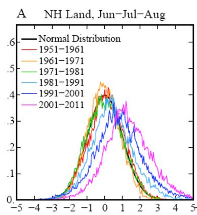
This shows the rightward spread of temperature deviations. The x-axis is in standard deviations, which makes the various geographies easily comparable (a hot day in Alaska is different from a hot day in Oklahoma). The authors define extreme heat as more than 3 standard deviations above the mean and note that the probability of extreme heat days has risen from less than 1% to above 10%.
One of the basic properties of the normal distribution is that, if X is distributed normally with mean µ and standard deviation s, then Y = A + bX is also distributed normally, with mean (A + bµ) and standard deviation bs. We will use this particularly when we "standardize" a sample: by subtracting its mean and dividing by its standard deviation, the result should be distributed with mean zero and standard deviation 1.
Oppositely, if we
are creating random variables with a standard deviation, we can take random
numbers with a N(0,1) distribution, multiply by the
desired standard deviation, and add the desired mean, to get normal random
numbers with any mean or standard deviation.
In Excel, you can create normally distributed random numbers by using
the RAND() function to generate
uniform random numbers on [0,1], then NORMSINV(
Motivation: Sample Averages are Normally Distributed
Before we do a long section on how to find areas under the normal distribution, I want to address the big question: Why we the heck would anybody ever want to know those?!?!
Consider a case where we have a population of people and we sample just a few to calculate an average. Before elections we hear about these types of procedures all of the time: a poll that samples just 1000 people is used to give information about how a population of millions of people will vote. These polls are usually given with a margin of error ("54% of people liked Candidate A over B, with a margin of error of plus or minus 2 percentage points"). If you don't know statistics then polls probably seem like magic. If you do know statistics then polls are based on a few simple formulas.
I have a dataset of about 206,639 people who reported their wage and salary to a particular government survey, the "Current Population Survey," the CPS. The true average of their wage and salaries was $19,362.62. (Not quite; the top income value is cut at $625,000 – people who made more are still just coded with that amount. But don't worry about that for now.) The standard deviation of the full 206,639 people is 39,971.91.
A histogram of the data shows that most people report zero (zero is the median value), which is reasonable since many of them are children or retired people. However some report incomes up to $625,000!
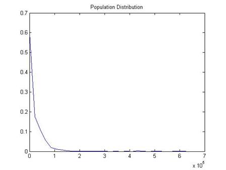
Taking an average of a population with such extreme values would seem to be difficult.
Suppose that I didn't want to calculate an average for all 206,639 people – I'm lazy or I've got a real old and slow computer or whatever. I want to randomly choose just 100 people and calculate the sample average. Would that be "good enough"?
Of course the first question is "good enough for what?" – what are we planning to do with the information?
But we can still ask whether the answer will be very close to the true value. In this case we know the true value; in most cases we won't. But this allows us to take a look at how the sampling works.
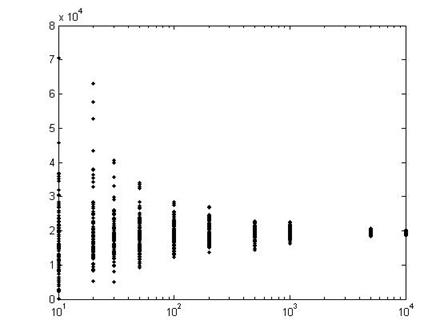
Here is a plot of values for 1000 different polls (each poll with just 100 people).
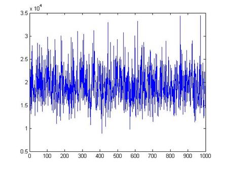
We can see that, although there are a few polls with averages as low almost 10,000 and a few with averages as high as 30,000, most of the polls are close to the true mean of $19,363.
In general the average of even a small sample is a good estimate of the true average value of the population. While a sample might pick up some extreme values from one side, it is also likely to pick extreme values from the other side, which will tend to balance out.
A histogram of the 1000 poll means is here:
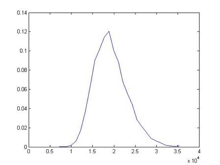
This shows that the distribution of the sample means looks like a Normal distribution – another case of how "normal" and ordinary the Normal distribution is.
Of course the size of each sample, the number of people in each poll, is also important. Sampling more people gets us better estimates of the true mean.
This graph shows the results from 100 polls, each with different sample sizes.
In the first set of 100 polls, on the left, each poll has just 10 people in it, so the results are quite varied. The next set has 20 people in each poll, so the results are closer to the true mean. By the time we get to 100 people in each poll (102 on the log-scale x-axis), the variation in the polls is much smaller.
Each distribution has a bell shape, but we have to figure out if there is a single invariant distribution or only a family of related bell-shaped curves.
If we subtract the mean, then we can center the distribution around zero, with positive and negative values indicating distance from the center. But that still leaves us with different scalings: as the graph above shows, the typical distance from the center gets smaller. So we divide by its standard deviation and we get a "Standard Normal" distribution.
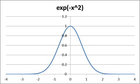
The Standard Normal graph is:
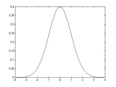
Note that it is symmetric around zero. Like any histogram, the area beneath the curve is a measure of the probability. The total area under the curve is exactly 1 (probabilities must add up to 100%). We can use the known function to calculate that the area under the curve, from -1 to 1, is 68.2689%. This means that just over 68% of the time, I will draw a value from within 1 standard deviation of the center. The area of the curve from -2 to 2 is 95.44997%, so we'll be within 2 standard deviations over 95.45% of the time.
It is important to be able to calculate areas under the Standard Normal. For this reason people used to use big tables (statistics textbooks still have them); now we use computers. But even the computers don't always quite give us the answer that we want, we have to be a bit savvy.
So the normal CDF of, say, -1, is the area under the pdf of the points to the left of -1:
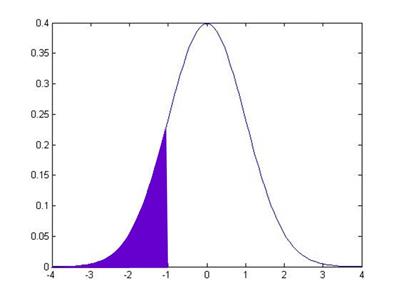
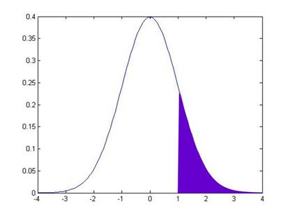
This area is 15.87%. How can I use this information to get the value that I earlier told you, that the area in between -1 and 1 is 68.2689%? Well, we know two other things (more precisely, I know them and I wrote them just 3 paragraphs up, so you ought to know them). We know that the total area under the pdf is 100%. And we know that the pdf is symmetric around zero. This symmetry means that the area under the other tail, the area from +1 all the way to the right, is also 15.87%.
So to find the area in between -1 and +1, I take 100% and subtract off the two tail areas:
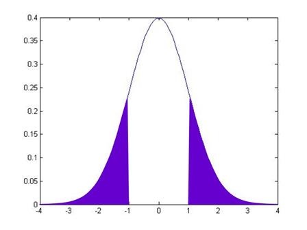
And this middle area is 100 – 15.87 – 15.87 = 68.26.
Sidebar: you can
think of all of this as "adding up" without calculus. On the other hand, calculus makes this
procedure much easier and we can precisely define the cdf
as the integral, from negative infinity to some point Z, under the pdf: ![]() .
.
So with just this simple knowledge, you can calculate all sorts of areas using just the information in the CDF.
Hints on
using Excel, SPSS, and Matlab to calculate the Standard Normal
cdf
Excel
Excel has both normdist and normsdist. For normdist, you need to tell it the mean and standard deviation, so use the function normdist(X,mean,stdev,cumulative). For normsdist it assumes the mean is zero and standard deviation is one so you just use normsdist(X). Read the help files to learn more. The final argument of the normdist function, "Cumulative" is a true/false: if true then it calculates the cdf (area to the left of X); if false it calculates the pdf. [Personally, that's an ugly and non-intuitive bit of coding, but then again, Microsoft has no sense of beauty.]
To figure out the
other way – what X value gives me some particular probability, we use norminv or normsinv.
All of these
commands are under "Insert"
then "Function"
then, under "Select a Category" choose "Statistical".
Mistress Google knows all. When I google "Normal cdf calculator" I get a link to http://www.uvm.edu/~dhowell/StatPages/More_Stuff/normalcdf.html. This is a simple and easy interface: put in the z-value to get the probability area or the inverse. Even ask Siri!
SPSS
For SPSS you can open it up with an empty dataset and go to the "Data View" tab. Then use "Transform," "Compute Variable…" and, under "Function Group" find "CDF and Noncentral CDF". Then "Cdf.Normal(X,mean,stdev)" calculates the normal cdf for the given X variable. Select this function and use the up-arrow to push it into the "Numeric Expression" dialog box. For any of the inputs (which SPSS denotes as "?") you can click on a variable from the list on the left. Or just type in the values. You need to give your output variable a name, this is the blank "Target Variable" on the upper left-hand side. If you're just doing calculations then give it any name; later on, if you are doing more complex series of calculations, you can worry about understandable variable names. Then hit "OK" and look back in the "Data View." (It will spawn an Output view but that only tells you if there were errors in the function.)
To go backwards, find "Inverse DF" under "Function Group" and then "IDF.Normal(p,mean,stdev)" where you input the probability.
Matlab
Matlab has the command, normcdf(X,mean,stdev). The inputs mean and stdev are the mean and standard deviations of the normal distribution considered; for the Standard Normal you can just leave those blank and just write normcdf(X). If X is a vector or matrix then it computes the standard normal cdf of each cell value. The function normpdf(X,mean,stdev) is the pdf naturally.
Norminv(p,mean,stdev) gives the inverse of the normcdf function and normsinv(p) gives the inverse for the standard normal.
R
For the cumulative distribution R uses pnorm(X,mean,stdev)although you can omit mean and stdev if you want 0 and 1 values. For the pdf use dnorm(X,mean,stdev). The inverse (quantiles) can be found from qnorm(p,mean,stdev).
Side Note: The basic
property, that the distribution is normal whatever the time interval, is what
makes the normal distribution {and related functions, called Lévy distributions} special. Most distributions would not have this
property so daily changes could have different distributions than weekly,
monthly, quarterly, yearly, or whatever!
Recall from
calculus the idea that some functions are not differentiable in places – they
take a turn that is so sharp that, if we were to approximate the slope of the
function coming at it from right or left, we would get very different
answers. The function,
![]() , is an example: at zero the left-hand derivative is -1; the
right-hand derivative is 1. It is not
differentiable at zero – it turns so sharply that it cannot be well
approximated by local values. But it is
continuous – it can be continuous even if it is not differentiable.
, is an example: at zero the left-hand derivative is -1; the
right-hand derivative is 1. It is not
differentiable at zero – it turns so sharply that it cannot be well
approximated by local values. But it is
continuous – it can be continuous even if it is not differentiable.
Now suppose I had a function that was everywhere continuous but nowhere differentiable – at every point it turns so sharply as to be unpredictable given past values. Various such functions have been derived by mathematicians, who call it a Wiener process (it generates Brownian motion). (When Einstein visited CCNY in 1905 he discussed his paper using Brownian motion to explain the movements of tiny particles in water, that are randomly bumped around by water molecules.) This function has many interesting properties – including an important link with the Normal distribution. The Normal distribution gives just the right degree of variation to allow continuity – other distributions would not be continuous or would have infinite variance.
Note also that a Wiener process has geometric form that is independent of scale or orientation – a Wiener process showing each day in the year cannot be distinguished from a Wiener process showing each minute in another time frame. As we noted above, price changes for any time interval are normal, whether the interval is minutely, daily, yearly, or whatever. These are fractals, curious beasts described by mathematicians such as Mandelbrot, because normal variables added together are still normal. (You can read Mandelbrot's 1963 paper in the Journal of Business, which you can download from JStor – he argues that Wiener processes are unrealistic for modeling financial returns and proposes further generalizations.)
The Normal
distribution has a
pdf which looks ugly but isn't so bad once you break it down. It is proportional to ![]() . This is what gives
it a bell shape:
. This is what gives
it a bell shape:
To make this a real probability we need to have all of its area sum up to one, so the probability density function (PDF) for a standard normal (with zero mean and standard deviation of one) is
![]() .
.
To allow a mean, µ, different from zero and a standard deviation, σ, different from one, we modify the formula to this:
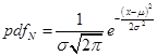 .
.
The connection with e is useful if it reminds you of when you learned about "natural logarithms" and probably thought "what the heck is 'natural' about that ugly thing?!" But you learn that it comes up everywhere (think it's bad now? wait for differential equations!) and eventually make your peace with it. So too the 'normal' distribution.
If you think that
the PDF is ugly then don't feel bad – its discoverer didn't like it
either. Stigler's History of Statistics
relates that Laplace first derived the function as the limit of a binomial
distribution as ![]() but couldn't believe
that anything so ugly could be true. So
he put it away into a drawer until later when Gauss derived the same formula
(from a different exercise) – which is why the Normal distribution is often
referred to as "Gaussian". The
Normal distribution arises in all sorts of other cases: solutions to partial
differential equations; in physics Maxwell used it to describe the diffusion of
gases or heat (again Brownian motion); in information theory where it is
connected to standard measures of entropy (Kullback Liebler); even in the distribution of prime factors in
number theory, the Erdős–Kac
Theorem.
but couldn't believe
that anything so ugly could be true. So
he put it away into a drawer until later when Gauss derived the same formula
(from a different exercise) – which is why the Normal distribution is often
referred to as "Gaussian". The
Normal distribution arises in all sorts of other cases: solutions to partial
differential equations; in physics Maxwell used it to describe the diffusion of
gases or heat (again Brownian motion); in information theory where it is
connected to standard measures of entropy (Kullback Liebler); even in the distribution of prime factors in
number theory, the Erdős–Kac
Theorem.
Finally I'll note the statistical quincunx, which is a great word since it sounds naughty but is actually geeky (google it or I'll try to get an online version to play in class).
Estimating Parameters
Learning Outcomes (from CFA exam Study Session 3, Quantitative Methods)
Students will be able to:
§ define the standard normal distribution, explain how to
standardize a random variable, and calculate and interpret probabilities using
the standard normal distribution;
The sample average has a normal distribution. This is hugely important for two reasons: one, it allows us to estimate a parameter, and two, because it allows us to start to get a handle on the world and how we might be fooled.
Estimating a parameter
The basic idea is that if we take the average of some sample of data, this average should be a good estimate of the true mean. For many beginning students this idea is so basic and obvious that you never think about when it is a reasonable assumption and when it might not be. For example, one of the causes of the Financial Crisis was that many of the 'quants' (the quantitative modelers) used overly-optimistic models that didn't seriously take account of the fact that financial prices can change dramatically. Most financial returns are not normally distributed! But we'll get more into that later; for now just remember this assumption. Later we'll talk about things like bias and consistency.
Variation around central mean
Knowing that the sample average has a normal distribution also helps us specify the variation involved in the estimation. We often want to look at the difference between two sample averages, since this allows us to tell if there is a useful categorization to be made: are there really two separate groups? Or do they just happen to look different?
How can we try to guard against seeing relationships where, in fact, none actually exist?
To answer this question we must think like statisticians. To "think like a statistician" is to do mental handstands; it often seems like looking at the world upside-down. But as you get used to it, you'll discover how valuable it is. (There is another related question: "What if there really is a relationship but we don't find evidence in the sample?" We'll get to that.)
The first step in "thinking like a statistician" is to ask, What if there were actually no relationship; zero difference? What would we see?
Consider two
random variables, X and Y; we want to see if there is a difference in mean
between them. We know that the sample
averages are distributed normally so both ![]() and
and ![]() are distributed
normally. We know additionally that
linear functions of normal distributions are normal as well, so
are distributed
normally. We know additionally that
linear functions of normal distributions are normal as well, so ![]() is distributed
normally. If there were no difference
in the means of the two variables then
is distributed
normally. If there were no difference
in the means of the two variables then ![]() would have a true mean
of zero;
would have a true mean
of zero; ![]() . But we are not
likely to ever see a sample mean of exactly zero! Sometimes we will probably see a positive
number, sometimes a negative. How big of
a difference would convince us? A big
difference would be evidence in favor of different means; a small difference
would be evidence against. But, in the
phrase of Dierdre McCloskey, "How big is
big?"
. But we are not
likely to ever see a sample mean of exactly zero! Sometimes we will probably see a positive
number, sometimes a negative. How big of
a difference would convince us? A big
difference would be evidence in favor of different means; a small difference
would be evidence against. But, in the
phrase of Dierdre McCloskey, "How big is
big?"
Let's do an example. X and Y are both distributed normally but with a moderately error relative to their mean (a modest signal-to-noise ratio), so X~N(10,3) and Y~N(12,3), with 50 observations.
In our sample the
difference is 0.95; ![]() =-0.95.
=-0.95.
A histogram of these differences shows:
Now we consider a rather strange thing: suppose that there were actually zero difference – what might we see? On the Excel sheet "normal_differences" (nothin' fancy) we look at 1000 repetitions of a sample of 50 observations of X and Y.
A histogram of 1000 possible samples in the case where there was no difference shows this:
So a difference of -0.95 is smaller than all but 62 of the 1000 random tries. We can say that, if there were actually no difference between X and Y, we would get something from the range of values above. Since we actually estimated -0.95, which is smaller than 62 of 1000, we could say that "there is just a 6.2% chance that X and Y could really have no difference but we'd see such a small value."
Law of Large Numbers
Probability and Statistics have many complications with twists and turns, but it all comes down to just a couple of simple ideas. These simple ideas are not necessarily intuitive – they're not the sort of things that might, at first, seem obvious. But as you get used to them, they'll become your friend.
With computers we can take much of the complicated formulas and derivations and just do simple experiments. Of course an experiment cannot replace a formal proof, but for the purposes of this course you don't need to worry about a formal proof.
One basic idea of statistics is the "Law of Large Numbers" (LLN). The LLN tells us that certain statistics (like the average) will very quickly get very close to the true value, as the size of the random sample increases. This means that if I want to know, say, the fraction of people who are right-handed or left-handed, or the fraction of people who will vote for Politician X versus Y, I don't need to talk with every person in the population.
This is strenuously counter-intuitive. You often hear people complain, "How can the pollsters claim to know so much about voting? They never talked to me!" But they don't have to talk to everyone; they don't even have to talk with very many people. The average of a random sample will "converge" to the true value in the population, as long as a few simple assumptions are satisfied.
Instead of a proof, how about an example? Open an Excel spreadsheet (or OpenOffice Calc, if you're an open-source kid). We are going to simulate the number of people who prefer politician X to Y.
We can do this
because Excel has a simple function, RAND(), which
picks a random number between 0 and 1.
So in the first cell,A1, I type "=
Assume that there are 1000 people in the population, so copy and paste the contents of cells A1 and B1 down to all of the cells A2 through A1000 and B2 through B1000. Now this gives us 1000 people, who are randomly assigned to prefer either politician X or Y. In B1001 you can enter the formula "=SUM(B1:B1000)" which will find out how many people (of 1000) who would vote for Politician X. Go back to cell C1 and enter the formula "=B1001/1000" – this tells you the fraction of people who are actually backing X (not quite equal to the percentage that you set at the beginning, but close).
Next suppose that we did a survey and randomly selected just 30 people for our poll. We know that we won't get the exact right answer, but we want to know "How inaccurate is our answer likely to be?" We can figure that out; again with some formulas or with some computing power.
For my example
(shown in the spreadsheet, samples_for_polls.xls) I first randomly select one
of the people in the population with the formula, in cell A3, =ROUND(1+RAND()*999,0). This takes a random number between 0 and 1 (RAND()), multiplies it by 999 so that I
will have a random number between 0 and 999, then adds 1 to get a random number
between 1 and 1000. Then it rounds it
off to be an integer (that's the =ROUND( ,0) part).
Next in B3 I write the formula, =INDIRECT(CONCATENATE("population!B",A3)). The inner part, CONCATENATE("population!B",A3), takes the random number that we generated in column A and makes it into a cell reference. So if the random number is 524 then this makes a cell address, population!B524. Then the =INDIRECT(population!B524) tells Excel to operate on it as if it were a cell address and return the value in B524 or the worksheet that I labeled "population".
On the worksheet I then copied these formulas down from A2 to B32 to get a poll of the views of 30 randomly-selected people. Then cell B1 gets the formula, =SUM(B3:B32)/30. This tells me what fraction of the poll support the candidate, if the true population has 45% support. I copied these columns five times to create 5 separate polls. When I ran it (the answers will be different for you), I got 4 polls showing less than 50% support (in a vote, that's the relevant margin) and 1 showing more than 50% support, with a rather wide range of values from 26% to 50%. (If you hit "F9" you will get a re-calculation, which takes a new bunch of random numbers.)
Clearly just 30 people is not a great poll; a larger poll would be more accurate. (Larger polls are also more expensive so polling organizations need to strategize to figure out where the marginal cost of another person in the poll equals the marginal benefit.)
In the problem set, you will be asked to do some similar calculations. If you have some basic computer programming background then you can use a more sophisticated program to do it (to create histograms and other visuals, perhaps). Excel is a donkey – it does the task but slowly and inelegantly.
So we can formulate many different sorts of questions once we have this figured out.
First the question of polls: if we poll 500 people to figure out if they approve or disapprove of the President, what will be the standard error?
With some math (![]() ) we can
figure out a formula for the standard error of the sample average. It is just the standard deviation of the
sample divided by the square root of the sample size. So the sample average is distributed normally
with mean of µ and standard error of
) we can
figure out a formula for the standard error of the sample average. It is just the standard deviation of the
sample divided by the square root of the sample size. So the sample average is distributed normally
with mean of µ and standard error of ![]() . This is sometimes
written compactly as
. This is sometimes
written compactly as ![]() .
.
Sometimes this
causes confusion because in calculating the standard error, s, we divided by
the square root of (N-1), since  , so it seems you're dividing twice. But this is correct: the first division gets
us an estimate of the sample's standard deviation; the second division by the
square root of N gets us the estimate of the sample average's standard error.
, so it seems you're dividing twice. But this is correct: the first division gets
us an estimate of the sample's standard deviation; the second division by the
square root of N gets us the estimate of the sample average's standard error.
The standardized
test statistic (sometimes called Z-score since Z will have a standard normal
distribution) is the mean divided by its standard error,  . This shows clearly
that a larger sample size (bigger N) amplifies differences of
. This shows clearly
that a larger sample size (bigger N) amplifies differences of ![]() from zero (the usual
null hypothesis). A small difference,
with only a few observations, could be just chance; a small difference,
sustained over many observations, is less likely to be just chance.
from zero (the usual
null hypothesis). A small difference,
with only a few observations, could be just chance; a small difference,
sustained over many observations, is less likely to be just chance.
One of the first
things to note about this formula is that, as N rises (as the sample gets
larger) the standard error gets smaller – the estimator gets more precise. So if N could rise towards infinity then the
sample average would converge to the true mean; we write this as ![]() where the
where the ![]() means "converges
in probability as N goes toward infinity".
means "converges
in probability as N goes toward infinity".
So the sample average is unbiased. This simply means that it gets closer and closer to the true value as we get more observations. Generally "unbiased" is a good thing, although later we'll discuss tradeoffs between bias and variance.
Return to the
binomial distribution, and its normal approximation. We know that std
error has its maximum when p= ½, so if we put in p=0.5 then the standard error
of a poll is, at worst, ![]() , so more observations give a better approximation. See Excel sheet poll_examples. We'll return to this once we learn a bit more
about the standard error of means.
, so more observations give a better approximation. See Excel sheet poll_examples. We'll return to this once we learn a bit more
about the standard error of means.
 A
bit of Math:
A
bit of Math:
We want to use our basic knowledge of linear combinations of normally-distributed variables to show that, if a random variable, X, comes from a normal distribution then its average will have a normal distribution with the same mean and the standard deviation of the sample divided by the square root of the sample size,
![]() .
.
The formula for
the average is ![]() . Consider first a
case where there are just 2 observations.
This case looks very similar to our rule about, if
. Consider first a
case where there are just 2 observations.
This case looks very similar to our rule about, if ![]() , then
, then ![]() . With N=2, this is
. With N=2, this is ![]() , which has mean
, which has mean ![]() , and since each X observation comes from the same
distribution then
, and since each X observation comes from the same
distribution then ![]() so the mean is
so the mean is ![]() (it's unbiased). You can work it out when there are
(it's unbiased). You can work it out when there are ![]() observations.
observations.
Now the standard
error of the mean is  . The covariance is
zero because we assume that we're making a random sample. Again since they come from the same
distribution,
. The covariance is
zero because we assume that we're making a random sample. Again since they come from the same
distribution, ![]() , the standard error
is
, the standard error
is ![]() .
.
With n
observations, the mean works out the same and the standard error of the average
is 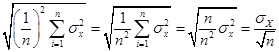 .
.
Hypothesis
Testing
Learning Outcomes (from CFA exam Study
Session 3, Quantitative Methods)
Students will be able to:
§ construct and interpret a confidence interval for a
normally distributed random variable, and determine the probability that a
normally distributed random variable lies inside a given confidence interval;
§ define the standard normal distribution, explain how to
standardize a random variable, and calculate and interpret probabilities using
the standard normal distribution;
§ explain the construction of confidence intervals;
§ define a hypothesis, describe the steps of hypothesis
testing, interpret and discuss the choice of the null hypothesis and
alternative hypothesis, and distinguish between one-tailed and two-tailed tests
of hypotheses;
§ define and interpret a test statistic, a Type I and a
Type II error, and a significance level, and explain how significance levels
are used in hypothesis testing;
Hypothesis
Testing
One of the
principal tasks facing the statistician is to perform hypothesis tests. These are a formalization of the most basic
questions that people ask and analyze every day – just contorted into odd
shapes. But as long as you remember the
basic common sense underneath them, you can look up the precise details of the
formalization that lays on top.
The basic
question is "How likely is it, that I'm being fooled?" Once we accept that the world is random
(rather than a manifestation of some god's will), we must decide how to make
our decisions, knowing that we cannot guarantee that we will always be
right. There is some risk that the world
will seem to be one way, when actually it is not. The stars are strewn randomly across the sky
but some bright ones seem to line up into patterns. So too any data might sometimes line up into
patterns.
A formal
hypothesis sets a mathematical condition that I want to test. Often this condition takes the form of some
parameter being zero for no relationship or no difference.
Statisticians
tend to stand on their heads and ask: What if there were actually no relationship? (Usually they ask questions of the form,
"suppose the conventional wisdom were true?") This statement, about "no
relationship," is called the Null
Hypothesis, sometimes abbreviated as H0. The Null Hypothesis is tested against an Alternative Hypothesis, HA.
Before we even
begin looking at the data we can set down some rules for this test. We know that there is some probability that
nature will fool me, that it will seem as though there is a relationship when
actually there is none. The statistical
test will create a model of a world where there is actually no relationship and
then ask how likely it is that we could see what we actually see, "How
likely is it, that I'm being fooled?"
The
"likelihood that I'm being fooled" is the p-value.
For a scientific
experiment we typically first choose the level of certainty that we
desire. This is called the significance
level. This answers, "How low does
the p-value have to be, for me to accept the formal hypothesis?" To be fair, it is important that we set this
value first because otherwise we might be biased in favor of an outcome that we
want to see. By convention, economists
typically use 10%, 5%, and 1%; 5% is the most common.
A five percent
level of a test is conservative, it means that we want to see so much evidence
that there is only a 5% chance that we could be fooled into thinking that
there's something there, when nothing is actually there. Five percent is not perfect, though – it
still means that of every 20 tests where I decide that there is a relationship
there, it is likely that I'm being fooled in one of those – I'm seeing a
relationship where there's nothing there.
To help ourselves
to remember that we can never be truly certain of our judgment of a test, we
have a peculiar language that we use for hypothesis testing. If the "likelihood that I'm being
fooled" is less than 5% then we say that the data allow us to reject the
null hypothesis. If the "likelihood
that I'm being fooled" is more than 5% then the data do not reject the
null hypothesis.
Note the
formalism: we never "accept" the null hypothesis. Why not?
Suppose I were doing something like measuring a piece of machinery,
which is supposed to be a centimeter long.
The null hypothesis is that it is not defective and so is one centimeter
in length. If I measure with a ruler I
might not find any difference to the eye.
So I cannot reject the hypothesis that it is one centimeter. But if I looked with a microscope I might
find that it is not quite one centimeter!
The fact that, with my eye, I don't see any difference, does not imply
that a better measurement could not find any difference. So I cannot say that it is truly exactly one
centimeter; only that I can't tell that it isn't.
So too with
statistics. If I'm looking to see if
some portfolio strategy produces higher returns, then with one month of data I
might not see any difference. So I would
not reject the null hypothesis (that the new strategy is no improvement). But it is possible that the new strategy, if
carried out for 100 months or 1000 months or more might show some tiny
difference.
Not rejecting the
null is saying that I'm not sure that I'm not being fooled. (Read that sentence again; it's not
immediately clear but it's trying to make a subtle and important point.)
To summarize,
Hypothesis Testing asks, "What is the chance that I would see the value
that I've actually got, if there truly were no relationship?" If this p-value is lower than 5% then I
reject the null hypothesis of "no relationship." If the p-value is greater than 5% then I do
not reject the null hypothesis of "no relationship."
The rest is
mechanics.
The null
hypothesis would tell that a parameter has some particular value, say zero: ![]() ; the alternative hypothesis is
; the alternative hypothesis is ![]() . Under the null
hypothesis the parameter has some distribution (often normal), so
. Under the null
hypothesis the parameter has some distribution (often normal), so ![]() . Generally we have an
estimate for
. Generally we have an
estimate for ![]() ,
which is
,
which is ![]() (for small samples
this inserts additional uncertainty). So
I know that, under the null hypothesis,
(for small samples
this inserts additional uncertainty). So
I know that, under the null hypothesis, ![]() has a standard normal
distribution (mean of zero and standard deviation of one). I know exactly what this distribution looks
like, it's the usual bell-shaped curve:
has a standard normal
distribution (mean of zero and standard deviation of one). I know exactly what this distribution looks
like, it's the usual bell-shaped curve:
So from this I
can calculate, "What is the chance that I would see the value that I've
actually got, if there truly were no relationship?," by asking what is the
area under the curve that is farther away from zero than the value that the
data give. (I still don't know what
value the data will give! I can do all
of this calculation beforehand.)
Any particular
estimate of ![]() is generally going to be
is generally going to be ![]() . So the test
statistic is formed with
. So the test
statistic is formed with ![]() .
.
Looking at the
standard normal pdf, a value of the test statistic of 1.5 would not meet the 5%
criterion (go back and calculate areas under the curve). A value of 2 would meet the 5% criterion,
allowing us to reject the null hypothesis.
For a 5% significance level, the standard normal critical value is 1.96: if the test statistic is larger than 1.96
(in absolute value) then its p-value is less than 5%, and vice versa. (You can find critical values by looking them
up in a table or using the computer.)
Sidebar: Sometimes you see people
do a one-sided test, which is within the letter of the law but not necessarily
the spirit of the law (particularly in regression formats). It allows for less restrictive testing, as
long as we believe that we know that there is only one possible direction of
deviation (so, for example, if the sample could be larger than zero but never
smaller). But in this case maybe the normal
distribution is inapplicable.
The test
statistic can be transformed into measurements of ![]() or into a confidence
interval.
or into a confidence
interval.
If I know that I
will reject the null hypothesis of ![]() at a 5% level if the
test statistic,
at a 5% level if the
test statistic, ![]() , is greater than 1.96 (in absolute value), then I can change
around this statement to be about
, is greater than 1.96 (in absolute value), then I can change
around this statement to be about ![]() . This says that if
the estimated value of
. This says that if
the estimated value of ![]() is less than 1.96
standard errors from zero, we cannot reject the null hypothesis. So cannot reject if:
is less than 1.96
standard errors from zero, we cannot reject the null hypothesis. So cannot reject if:
![]()
![]()
![]() .
.
This range, ![]() , is directly comparable to
, is directly comparable to ![]() . If I divide
. If I divide ![]() by its standard error
then this ratio has a normal distribution with mean zero and standard deviation
of one. If I don't divide then
by its standard error
then this ratio has a normal distribution with mean zero and standard deviation
of one. If I don't divide then ![]() has a normal
distribution with mean zero and standard deviation,
has a normal
distribution with mean zero and standard deviation, ![]() .
.
If the null
hypothesis is not zero but some other number, ![]() , then under the null hypothesis the estimator would have a
normal distribution with mean of
, then under the null hypothesis the estimator would have a
normal distribution with mean of ![]() and standard error,
and standard error, ![]() . To transform this to
a standard normal would mean subtracting the mean and dividing by
. To transform this to
a standard normal would mean subtracting the mean and dividing by ![]() , so cannot reject if
, so cannot reject if ![]() , i.e. cannot reject if
, i.e. cannot reject if ![]() is within the range,
is within the range, ![]() .
.