Class Oct 3

Kevin R Foster, CCNY, ECO B2000

Fall 2013

Jumping into OLS

OLS is Ordinary Least Squares, which as the name implies is ordinary, typical, common – something that is widely used in just about every economic analysis.

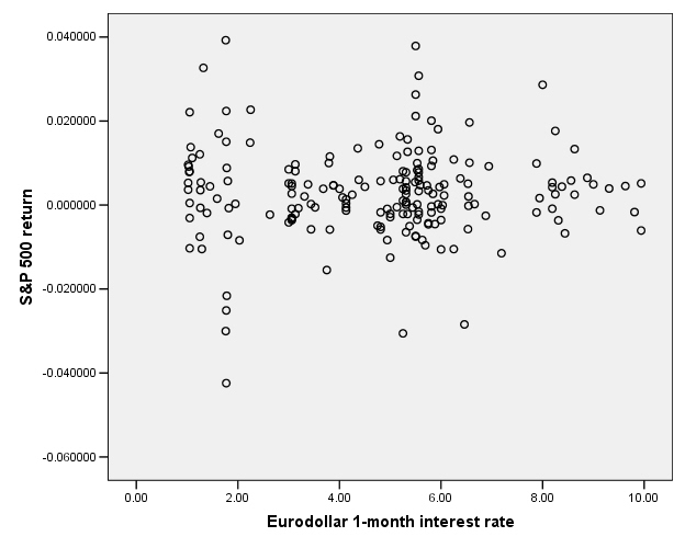
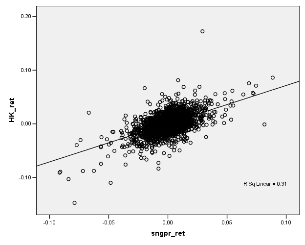
We are accustomed to looking at graphs that show values of two variables and trying to discern patterns. Consider again these two graphs of financial variables.

This plots the returns of Hong Kong's Hang Seng index against the returns of Singapore's Straits Times index (over the period from Jan 2, 1991 to Jan 31, 2006)

This next graph shows the S&P 500 returns and interest rates (1-month Eurodollar) during 1989-2004.

You don't have to be a highly-skilled econometrician to see the difference in the relationships. It would seem reasonable that the Hong Kong and Singapore stock indexes are closely linked while the US stock index is not closely related to interest rates.

So we want to ask, how could we measure these relationships? Since these two graphs are rather extreme cases, how can we distinguish cases in the middle? How can we try to guard against seeing relationships where, in fact, none actually exist? We will consider each of these questions in turn.

How can we measure the relationship?

Facing a graph like the Hong Kong/Singapore stock indexes, we might represent the relationship by drawing a line, something like this:

Now if this line-drawing were done just by hand, just sketching in a line, then different people would sketch different lines, which would be clearly unsatisfactory. What is the process by which we sketch the line?

Typically we want to find a relationship because we want to predict something, to find out that, if I know one variable, then how does this knowledge affect my prediction of some other variable. We call the first variable, the one known at the beginning, X. The variable that we're trying to predict is called Y. So in the example above, the Singapore stock index is X and the Hong Kong index is Y. The line that we would draw in the picture would represent our best guess of what Y would be, given our knowledge about X.

This line is drawn to get the best guess "close to" the actual Y values – where by "close to" we actually minimize the average squared distance. Why square the distance? This is one question which we will return to, again and again; for now the reason is that a squared distance really penalizes the big misses. If I square a small number, I get a bigger number. If I square a big number, I get a HUGE number. (And if I square a number less than one, I get a smaller number.) So minimizing the squared distance will mean that I am willing to make a bunch of small errors in order to reduce a really big error. This is why there is the "LS" in "OLS" -- "Ordinary Least Squares" finds the least squared difference.

A computer can easily calculate a line that minimizes the squared distance between each Y value and the best prediction. There are also formulas for it. (We'll come back to the formulas; put a lightning bolt here to remind us: .)

For a moment consider how powerful this procedure is. A line that represents a relationship between X and Y can be entirely produced by knowing just two numbers: the y-intercept and the slope of the line. In algebra class you probably learned the equation as:

where the slope is and the y-intercept is . When then , which is the value of the line when the line intersects the Y-axis (when X is zero). The y-intercept can be positive or negative or zero. The slope is the value of , which tells how much Y changes when X changes by one unit. To find the predicted value of Y at any point we substitute the value of X into the equation.

In econometrics we will typically use a different notation,

where now is the y-intercept and the slope is . (Econometricians looooove Greek letters like beta, get used to it!)

The relationship between X and Y can be positive or negative. Basic economic theory says that we expect that the amount demanded of some item will be a positive function of income and a negative function of price (for a normal good). We can easily have a case where .

If X and Y had no systematic relation, then this would imply that (in which case, is just the mean of Y). In the case, Y takes on higher or lower values independently of what is the level of X.

This is the case for the S&P 500 return and interest rates:

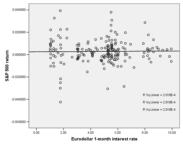
So there does not appear to be any relationship.

Let's fine up the notation from above a bit more: when we fit a line to the data, we do not always have Y exactly and precisely equal to . Sometime Y is a bit bigger, sometimes a bit smaller. The difference is an error in the model. So we should actually write where epsilon is the error between the model value of Y and the actual observed value.

Computer programs will easily compute this OLS line; even Excel will do it. When you create an XY (Scatter) chart, then right-click on the data series, "Add Trendline" and choose "Linear" to get the OLS estimates.

Other Notation:

There is another possible notation, that . This is often implicit in discussions of hedge funds or financial investing. If X is the return on the broad market (the S&P500, for example) and Y is the return of a hedge fund, then the hedge fund managers must make a case that they can provide "alpha" – that for their hedge fund . This implies that no matter what the market return is, the hedge fund will return better. The other desirable case is for a hedge fund with beta near zero – which might seem odd at first. But this provides diversification: a low beta means that the fund returns do not really depend on the broader market. An investment with a zero beta and alpha of 0.5% is a savings account. An investment promising zero beta and alpha of 20% is a fraud.

Another Example

This representation is powerful because it neatly and compactly summarizes a great deal of underlying variation. Consider the case of looking at the time that people spend eating and drinking, as reported in the ATUS data; we want to see if there is a relationship with the person's age. If we compute averages for each age (average time spent by people who are 18 years old, average time spent by people who are 19 years old, 20 years old, etc – all the way to 85 years old) along with the standard errors we get this chart:

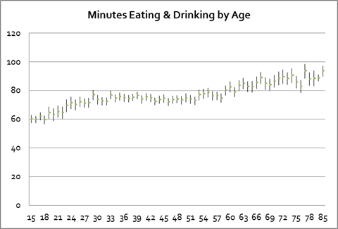
There seems to be an upward trend although we might distinguish a flattening of time spent, between ages 30 and 60. But all of this information takes a table of numbers with 67 rows and 4 columns s0 268 separate numbers! If we represent this as just a line then we need just two numbers, the intercept and the slope. This also makes more effective use of the available information to "smooth out" the estimated relationship. (For instance, there is a leap up for 29-year-olds but then a leap back down – do we really believe that there is really that sort of discontinuity or do we think this could just be the randomness of the data? A fitted line would smooth out that bump.)

How can we distinguish cases in the middle?

Hopefully you've followed along so far, but are currently wondering: How do I tell the difference between the Hong Kong/Singapore case and the S&P500/Interest Rate case? Maybe art historians or literary theorists can put up with having "beauty" as a determinant of excellence, but what is a beautiful line to econometricians?

There are two separate answers here, and it's important that we separate them. Many analyses muddle them up. One answer is simply whether the line tells us useful information. Remember that we are trying to estimate a line in order to persuade (ourselves or someone else) that there is a useful relationship here. And "useful" depends crucially upon the context. Sometimes a variable will have a small but vital relationship; others may have a large but much less useful relation. To take an example from macroeconomics, we know that the single largest component of GDP is consumption, so consumption has a large impact on GDP. However US consumption is based on the individual choices of 300m people, so it's difficult for policymakers to have a direct and immediate effect upon it. Beginning students are often surprised to discover how important an effect inventory investment has historically had on US GDP growth, even though inventory adjustments are a tiny slice of GDP. The Fed's actions have a tiny direct effect yet we all agree that they are very important because this tiny effect may help the economy in huge ways.

This first question, does the line persuade, is always contingent upon the problem at hand; there is no easy answer. You can only learn this by reading other people's analyses and by practicing on your own. It is an art form to be learned, but the second part is science.

The economist Dierdre McCloskey has a simple phrase, "How big is big?" This is influenced by the purpose of the research and the aim of discovering a relation: if we want to control some outcome or want to predict the value of some unknown variable or merely to understand a relationship.

The first question, about the usefulness and persuasiveness of the line, also depends on the relative sizes of the modeled part of Y and the error. Returning to the notation introduced, this means the relative sizes of the predictable part of Y, , versus the size of . As epsilon gets larger relative to the predictable part, the usefulness of the model declines.

The second question, about how to tell how well a line describes data, can be answered directly with statistics, and it can be answered for quite general cases.

How can we try to guard against seeing relationships where, in fact, none actually exist?

To answer this question we must think like statisticians, do mental handstands, look at the world upside-down.

Remember, the first step in "thinking like a statistician" is to ask, What if there were actually no relationship; zero relationship (so )? What would we see?

If there were no relationship then Y would be determined just by random error, unrelated to X. But this does not automatically mean that we would estimate a zero slope for the fitted line. In fact we are highly unlikely to ever estimate a slope of exactly zero. We usually assume that the errors are symmetric, i.e. if the actual value of Y is sometimes above and sometimes below the modeled value, without some oddball skew up or down. So even in a case where there is actually a zero relationship between Y and X, we might see a positive or negative slope.

We would hope that these errors in the estimated slope would be small – but, again, "how small is small?"

Let's take another example. Suppose that the true model is Y = 10 + 2X (so and ). But of course there will be an error; let's consider a case where the error is pretty large. In this case we might see a set of points like this:

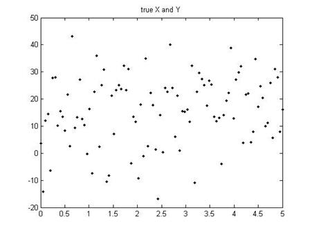
When we estimate the slope for those dots, we would find not 2 but, in this case (for this particular set of errors), 1.61813.

Now we consider a rather strange thing: suppose that there were actually zero relationship between X and Y (so that actually ). Next suppose that, even though there were actually zero relation, we tried to plot a line and so calculated our estimate of . To give an example, we would have the computer calculate some random numbers for X and Y values, then estimate the slope, and we would find 1.45097. Do it again, and we might get 0.36131. Do it 10,000 times (not so crazy, actually – the computer does it in a couple of seconds), and we'd find the following range of values for the estimated slope:

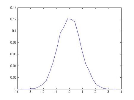
So our estimated slope from the first time, 1.61813, is "pretty far" from zero. How far? The estimated slope is farther than just 659 of those 10,000 tries, which is 6.59%.

So we could say that, if there were actually no relationship between X and Y, but we incorrectly estimated a slope, then we'd get something from the range of values shown above. Since we estimated a value of 1.61813, which is farther from zero than just 6.59% if there were actually no relationship, we might say that "there is just a 6.59% chance that X and Y could truly be unrelated but I'd estimate a value of 1.61813." [This is all based on a simple program in Matlab, emetrics1.m]

Now this is a more reasonable measure: "What is the chance that I would see the value, that I've actually got, if there truly were no relationship?" And this percentage chance is relevant and interesting to think about.

This formalization is "hypothesis testing". We have a hypothesis, for example "there is zero relation between X and Y," which we want to test. And we'd like to set down rules for making decisions so that reasonable people can accept a level of evidence as proving that they were wrong. (An example of not accepting evidence: the tobacco companies remain highly skeptical of evidence that there is a relationship between smoking and lung cancer. Despite what most researchers would view as mountains of evidence, the tobacco companies insist that there is some chance that it is all just random. They're right, there is "some chance" – but that chance is, by now, probably something less than 1 in a billion.) Most empirical research uses a value of 5% -- we want to be skeptical enough that there is only a 5% chance that there might really be no relation but we'd see what we saw. So if we went out into the world and did regressions on randomly chosen data, then in 5 out of 100 cases we would think that we had found an actual relation. It's pretty low but we still have to keep in mind that we are fallible, that we will go wrong 5 out of 100 (or 1 in 20) times.

Under some general conditions, the OLS slope coefficient will have a normal distribution -- not a standard normal, though, it doesn't have a mean of zero and a standard deviation of one.

However we can estimate its standard error and then can figure out how likely it is, that the true mean could be zero, but I would still observe that value.

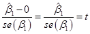
This just takes the observed slope value, call it (we often put "hats" over the variables to denote that this is the actual observed value), subtract the hypothesized mean of zer0, and divide by the standard error:

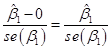
We call this the "t-statistic". When we have a lot of observations, the t-statistic has approximately a standard normal distribution with zero mean and standard deviation of one.

For the careful students, note that the t-statistic actually has a t-distribution, which has a shape that depends on the number of observations used to construct it (the degrees of freedom). When the number of degrees of freedom is more than 30 (which is almost all of the time), the t-distribution is just about the same as a normal distribution. But for smaller values the t-distribution has fatter tails.

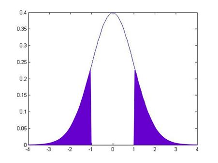
The t-statistic allows us to calculate the probability that, if there were actually a zero relationship, I might actually observe a value as extreme as . By convention we look at distance either above or below zero, so we want to know the probability of seeing a value as far from zero as either or . If were equal to 1, then this would be:

while if were another value, it would be:

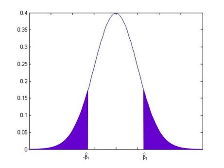
From working on the probabilities under the standard normal, you can calculate these areas for any given value of .

In fact, these probabilities are so often needed, that most computer programs calculate them automatically – they're called "p-values". The p-value gives the probability that the true coefficient could be zero but I would still see a number as extreme as the value actually observed. By convention we refer to slopes with a p-value of 0.05 or less (less than 5%) as "statistically significant".

(We can test if coefficients are different from other values than just zero, but for now that is the most common so we focus on it.)

Confidence Intervals for Regression Estimates

There is another way of looking at statistical significance. We just reviewed the procedure of taking the observed value, subtracting off the mean, dividing by the standard error, and then comparing the calculated t-statistic against a standard normal distribution.

But we could do it backwards, too. We know that the standard normal distribution has some important values in it, for example the values that are so extreme, that there is just a 5% chance that we could observe what we saw, yet the true value were actually zero. This 5% critical value is just below 2, at 1.96. So if we find a t-statistic that is bigger than 1.96 (in absolute value) then the slope would be "statistically significant"; if we find a t-statistic that is smaller than 1.96 (in absolute value) then the slope would not be "statistically significant". We can re-write these statements into values of the slope itself instead of the t-statistic.

We know from above that

,

and we've just stated that the slope is not statistically significant if:

.

This latter statement is equivalent to:

Which we can re-write as:

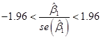
Which is equivalent to:

So this gives us a "Confidence Interval" – if we observe a slope within 1.96 standard errors of zero, then the slope is not statistically significant; if we observe a slope farther from zero than 1.96 standard errors, then the slope is statistically significant.

This is called a "95% Confidence Interval" because this shows the range within which the observed values would fall, 95% of the time, if the true value were zero. Different confidence intervals can be calculated with different critical values: a 90% Confidence Interval would need the critical value from the standard normal, so that 90% of the probability is within it (this is 1.64).

Details:

- statistical significance for a univariate regression is the same as overall regression significance – if the slope coefficient estimate is statistically significantly different from zero, then this is equivalent to the statement that the overall regression explains a statistically significant part of the data variation.

- Excel calculates OLS both as regression (from Data Analysis TookPak), as just the slope and intercept coefficients (formula values), and from within a chart

- There are important assumptions about the regression that must hold, if we are to interpret the estimated coefficients as anything other than within-sample descriptors:

o X completely specifies the causal factors of Y (nothing omitted)

o X causes Y in a linear manner

o errors are normally distributed

o errors have same variance even at different X (homoskedastic not heteroskedastic)

o errors are independent of each other

- Because OLS squares the residuals, a few oddball observations can have a large impact on the estimated coefficients, so must explore

Points:

Calculating the OLS Coefficients

The formulas for the OLS coefficients have several different ways of being written. For just one X-variable we can use summation notation (although it's a bit tedious). For more variables the notation gets simpler by using matrix algebra.

The basic problem is to find estimates of b₀ and b₁ to minimize the error in .

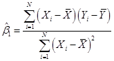
The OLS coefficients are found from minimizing the sum of squared errors, where each error is defined as so we want to . If you know basic calculus then you understand that you find the minimum point by taking the derivative with respect to the control variables, so differentiate with respect to b₀ and b₁. After some tedious algebra, find that the minimum value occurs when we use and , where:

.

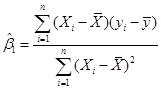
With some linear algebra, we define the equations as , where y is a column vector, , e is the same, , X is a matrix with a first column of ones and then columns of each X variable, 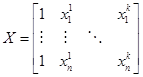, where there are k columns, and then . The OLS coefficients are then given as .

But the computer does the calculations so you only need these if you go on to become an econometrician.

To Recap:

· A zero slope for the line is saying that there is no relationship.

· A line has a simple equation, that Y = b₀ + b₁X

· How can we "best" find a value of b?

· We know that the line will not always fit every point, so we need to be a bit more careful and write that our observed Y values, Y_i (i=1, …, N), are related to the X values, X_i, as: Y_i = b₀ + b₁X_i + u_i. The u_i term is an error – it represents everything that we haven't yet taken into consideration.

· Suppose that we chose values for b₀ and b₁ that minimized the squared values of the errors. This would mean . This will generally give us unique values of b (as opposed to the eyeball method, where different people can give different answers).

· The b₀ term is the intercept and the b₁ term is the slope, .

· These values of b are the Ordinary Least Squares (OLS) estimates. If the Greek letters denote the true (but unknown) parameters that we're trying to estimate, then denote and as our estimators that are based on the particular data. We denote as the predicted value of what we would guess Yi would be, given our estimates of b₀ and b₁, so that .

· There are formulas that help people calculate and (rather than just guessing numbers); these are:

and

so that and

Why OLS? It has a variety of desirable properties, if the data being analyzed satisfy some very basic assumptions. Largely because of this (and also because it is quite easy to calculate) it is widely used in many different fields. (The method of least squares was first developed for astronomy.)

· OLS requires some basic assumptions:

o The conditional distribution of u_i given X_i has a mean of zero. This is a complicated way of saying something very basic: I have no additional information outside of the model, which would allow me to make better guesses. It can also be expressed as implying a zero correlation between X_i and u_i. We will work up to other methods that incorporate additional information.

o The X and e are i.i.d. This is often not precisely true; on the other hand it might be roughly right, and it gives us a place to start.

o X_i and u_i have fourth moments. This is technical and broadly true, whenever the X and Y data have a limit on the amount of variation, although there might be particular circumstances where it is questionable (sometimes in finance).

· These assumptions are costly; what do they buy us? First, if true then the OLS estimates are distributed normally in large samples. Second, it tells us when to be careful.

· Must distinguish between dependent and independent variables (no simultaneity).

· So if these are true then the OLS are unbiased and consistent. So and . The normal distribution, as the sample gets large, allows us to make hypothesis tests about the values of the betas. In particular, if you look back to the "eyeball" data at the beginning, you will recall that a zero value for the slope, b₁, is important. It implies no relationship between the variables. So we will commonly test the estimated values of b against a null hypothesis that they are zero.

· There are formulas that you can use, for calculating the standard errors of the b estimates, however for now there's no need for you to worry about them. The computer will calculate them. (Also note that the textbook uses a more complicated formula than other texts, which covers more general cases. We'll talk about that later.)