Class Oct 24

Kevin R Foster, CCNY, ECO B2000

Fall 2013

Multiple Regression – more than one X variable

Regressing just one variable on another can be helpful and useful (and provides a great graphical intuition) but it doesn't get us very far.

Consider this example, using data from the March 2010 CPS. We limit ourselves to only examining people with a non-zero annual wage/salary who are working fulltime (WSAL_VAL > 0 & HRCHECK = 2). We look at the different wages reported by people who label themselves as white, African-American, Asian, Native American, and Hispanic. There are 62,043 whites, 9,101 African-Americans, 4476 Asians, 2149 Native Americans, and 12,401 Hispanics in the data who fulfill this condition.

The average yearly salary for whites is $50,782; for African-Americans it is $39,131; for Asians $57,541; for Native Americans $38,036; for Hispanics it is $36,678. Conventional statistical tests find that these averages are significantly different. Does this prove discrimination? No; there are many other reasons why groups of people could have different incomes such as educational level or age or a multitude of other factors. (But it is not inconsistent with a hypothesis of racism: remember the difference, when evaluating hypotheses, between 'not rejecting' or 'accepting'). We might reasonably break these numbers down further.

These groups of people are different in a variety of ways. Their average ages are different between Hispanics, averaging 38.72 years, and non-Hispanics, averaging 42.41 years. So how much of the wage difference, for Hispanics, is due to the fact that they're younger? We could do an ANOVA on this but that would omit other factors.

The populations also different in gender ratios. For whites, 57% were male; for African-Americans 46% were male; for Hispanics 59% were male. Since gender also affects income, we might think some of the wage gap could be due, not to racial discrimination, but to gender discrimination.

But then they're also different in educational attainment! Among the Hispanic workers, 30% had not finished high school; for African-Americans 8.8% had not; for whites 9% had not finished with a diploma. And 12% of whites had an advanced degree while 8.3% of African Americans and 4.2% of Hispanics had such credentials. The different fractions in educational attainment add credibility to the hypothesis that not all racial/ethnic variation means discrimination (in the labor market, at least – there could be discrimination in education so certain groups get less or worse education).

Finally they're different in what section of the country they live in, as measured by Census region.

So how can we keep all of these different factors straight?

Multiple Regression in SPSS

From the standpoint of just using SPSS, there is no difference for the user between a univariate and multivariate linear regression. Again use "Analyze\ Regression\ Linear ..." but then add a bunch of variables to the "Independent(s)" box.

In formulas, model has k explanatory variables for each of observations (must have n > k)

Each coefficient estimate, notated as , has standardized distribution as t with (n – k) degrees of freedom.

Each coefficient represents the amount by which the y would be expected to change, for a small change in the particular x-variable (i.e. ).

Note that you must be a bit careful specifying the variables. The CPS codes educational attainment with a bunch of numbers from 31 to 46 but these numbers have no inherent meaning. So too race, geography, industry, and occupation. If a person graduates high school then their grade coding changes from 38 to 39 but this must be coded with a dummy variable. If a person moves from New York to North Dakota then this increases their state code from 36 to 38; this is not the same change as would occur for someone moving from North Dakota to Oklahoma (40) nor is it half of the change as would occur for someone moving from New York to North Carolina (37). Each state needs a dummy variable.

A multivariate regression can control for all of the different changes to focus on each item individually. So we might model a person's wage/salary value as a function of their age, their gender, race/ethnicity (African-American, Asian, Native American, Hispanic), if they're an immigrant, six educational variables (high school diploma, some college but no degree, Associate's in vocational field, Associate's in academic field, a 4-year degree, or advanced degree), if they're married or divorced/widowed/separated, if they're a union member, and if they're a veteran. Results (from the sample above, of March 2010 fulltime workers with non-zero wage), are given by SPSS as:

Model Summary
Model	R	R Square	Adjusted R Square	Std. Error of the Estimate
1	.454^a	.206	.206	46820.442
a. Predictors: (Constant), Veteran (any), African American, Education: Associate in vocational, Union member, Education: Associate in academic, Native American Indian or Alaskan or Hawaiian, Divorced or Widowed or Separated, Asian, Education: Advanced Degree, Hispanic, Female, Education: Some College but no degree, Demographics, Age, Education: 4-yr degree, Immigrant, Married, Education: High School Diploma

ANOVA^b
Model		Sum of Squares	df	Mean Square	F	Sig.
1	Regression	4.416E13	17	2.598E12	1185.074	.000^a
	Residual	1.704E14	77751	2.192E9
	Total	2.146E14	77768
a. Predictors: (Constant), Veteran (any), African American, Education: Associate in vocational, Union member, Education: Associate in academic, Native American Indian or Alaskan or Hawaiian, Divorced or Widowed or Separated, Asian, Education: Advanced Degree, Hispanic, Female, Education: Some College but no degree, Demographics, Age, Education: 4-yr degree, Immigrant, Married, Education: High School Diploma
b. Dependent Variable: Total wage and salary earnings amount - Person

Coefficients^a
Model		Unstandardized Coefficients		Standardized Coefficients	t	Sig.
Model		B	Std. Error	Beta	t	Sig.
1	(Constant)	10081.754	872.477		11.555	.000
	Demographics, Age	441.240	15.422	.104	28.610	.000
	Female	-17224.424	351.880	-.163	-48.950	.000
	African American	-5110.741	539.942	-.031	-9.465	.000
	Asian	309.850	819.738	.001	.378	.705
	Native American Indian or Alaskan or Hawaiian	-4359.733	1029.987	-.014	-4.233	.000
	Hispanic	-3786.424	554.159	-.026	-6.833	.000
	Immigrant	-3552.544	560.433	-.026	-6.339	.000
	Education: High School Diploma	8753.275	676.683	.075	12.936	.000
	Education: Some College but no degree	15834.431	726.533	.116	21.795	.000
	Education: Associate in vocational	17391.255	976.059	.072	17.818	.000
	Education: Associate in academic	21511.527	948.261	.093	22.685	.000
	Education: 4-yr degree	37136.959	712.417	.293	52.128	.000
	Education: Advanced Degree	64795.030	788.824	.400	82.141	.000
	Married	10981.432	453.882	.102	24.194	.000
	Divorced or Widowed or Separated	4210.238	606.045	.028	6.947	.000
	Union member	-2828.590	1169.228	-.008	-2.419	.016
	Veteran (any)	-2863.140	666.884	-.014	-4.293	.000
a. Dependent Variable: Total wage and salary earnings amount - Person

For the "Coefficients" table, the "Unstandardized coefficient B" is the estimate of , the "Std. Error" of the unstandardized coefficient is the standard error of that estimate, . (In economics we don't generally use the standardized beta, which divides the coefficient estimate by the standard error of X.) The "t" given in the table is the t-statistic, and "Sig." is its p-value – the probability, if the coefficient were actually zero, of seeing an estimate as large as the one that you got. (Go back and review if you don't remember all of the details of this.)

Multiple Regression in R

Again it’s not really different from a univariate regression. From the PUMS data, run these commands. First restrict to “prime age” working people (25-55 years old) and those with non-zero income, so

restrict1 <- ((dat1$AGE >= 25) & (dat1$AGE <= 55) & (dat1$INCWAGE > 0))

dat2 <- subset(dat1, restrict1)

summary(lm(INCWAGE ~ AGE + female + educ_hs + educ_somecoll + educ_collassoc + educ_coll + educ_adv, data=dat2))

The basic syntax is to ask R to give a summary of a lm (linear model) where INCWAGE is the Y-variable, explained by the rest of the list. Output is:

Call:

lm(formula = INCWAGE ~ AGE + female + educ_hs + educ_somecoll +

educ_collassoc + educ_coll + educ_adv, data = dat2)

Residuals:

Min 1Q Median 3Q Max

-121844 -28038 -8867 10608 585138

Coefficients:

Estimate Std. Error t value Pr(>|t|)

(Intercept) -1252.90 1140.15 -1.099 0.272

AGE 815.04 23.27 35.025 <2e-16 ***

female -19778.28 415.66 -47.583 <2e-16 ***

educ_hs 10370.50 750.73 13.814 <2e-16 ***

educ_somecoll 19969.80 795.61 25.100 <2e-16 ***

educ_collassoc 23035.49 967.20 23.817 <2e-16 ***

educ_coll 52716.51 727.83 72.429 <2e-16 ***

educ_adv 79187.87 771.38 102.657 <2e-16 ***

---

Signif. codes: 0 ‘***’ 0.001 ‘**’ 0.01 ‘*’ 0.05 ‘.’ 0.1 ‘ ’ 1

Residual standard error: 67600 on 106877 degrees of freedom

Multiple R-squared: 0.1511, Adjusted R-squared: 0.151

F-statistic: 2717 on 7 and 106877 DF, p-value: < 2.2e-16

A shortcut would use the “factor” type of data so:

summary(lm(INCWAGE ~ AGE + female + factor(educ_indx), data=dat2))

although you’d have to remember the coding of the education index.

A somewhat better specification might include some more variables and add in the heteroskedasticity-consistent errors, so

regression1 <- lm(INCWAGE ~ AGE + I(AGE^2) + female + factor(educ_indx) + africanamerican + nativeamerican + asianamerican+ Hispanic + raceother + kids_under5 + has_kids + non_citizen + veteran, data=dat2)

summary(regression1)

coeftest(regression1, df = Inf, vcov = vcovHC(regression1))

We'll often form hypotheses about regression coefficients: t-stats, p-values, and confidence intervals – so that's the same basic process as before. Usually two-sided (rarely one-sided).

We will commonly test if the coefficients 'are significant' – i.e. is there evidence in the data that the coefficient is different from zero? This goes back to our original example where we looked at the difference between the Hong Kong/Singapore stock returns and the US stock returns/interest rate. A zero slope is evidence against any relationship – this shows that the best guess of the value of Y does not depend on current information about the level of X. So coefficient estimates that are statistically indistinguishable from zero are not evidence that the particular X variable is useful in prediction.

A hypothesis test of some statistical estimate uses this estimator (call it ) and the estimator's standard error (denote it as ) to test against some null hypothesis value, . To make the hypothesis test, form , and – here is the magic! – under certain conditions this Z will have a Standard Normal distribution (or sometimes, if there are few degrees of freedom, a t-distribution; later in more advanced stats courses, some other distribution). The magic happens because if Z has a Standard Normal distribution then this allows me to measure if the estimate of X, , is very far away from . It's generally tough to specify a common unit that allows me to say sensible things about "how big is big?" without some statistical measure. The p-value of the null hypothesis tells me, "If the null hypothesis were actually true, how likely is it that I would see this value?" A low p-value tells me that it's very unlikely that my hypothesis could be true and yet I'd see the observed values, which is evidence against the null hypothesis.

Often the formula, , gets simpler when is zero, since it is just , and this is what SPSS prints out in the regression output labeled as "t". This generally has a t-distribution (with enough degrees of freedom, a Standard Normal) so SPSS calculates the area in the tails beyond this value and labels it "Sig".

This is in Chapter 5 of Stock & Watson.

We know that the standard normal distribution has some important values in it, for example the values that are so extreme, that there is just a 5% chance that we could observe what we saw, yet the true value were actually zero. This 5% critical value is just below 2, at 1.96. So if we find a t-statistic that is bigger than 1.96 (in absolute value) then the slope would be "statistically significant"; if we find a t-statistic that is smaller than 1.96 (in absolute value) then the slope would not be "statistically significant". We can re-write these statements into values of the slope itself instead of the t-statistic.

We know from above that

and we've just stated that the slope is not statistically significant if:

This latter statement is equivalent to:

Which we can re-write as:

Which is equivalent to:

So this gives us a "Confidence Interval" – if we observe a slope within 1.96 standard errors of zero, then the slope is not statistically significant; if we observe a slope farther from zero than 1.96 standard errors, then the slope is statistically significant.

This is called a "95% Confidence Interval" because this shows the range within which the observed values would fall, 95% of the time, if the true value were zero. Different confidence intervals can be calculated with different critical values: a 90% Confidence Interval would need the critical value from the standard normal, so that 90% of the probability is within it (this is 1.64).

A commonly overall assessment of the quality of the regression is the R² (displayed on the charts at the beginning automatically by SPSS). This is the fraction of the variance in Y that is explained by the model so 0 £ R² £ 1. Bigger is usually better, although different models have different expectations (i.e. it's graded on a curve).

Statistical Tests on Multiple Coefficients

Statistical significance of coefficient estimates is more complicated for multiple regression, we can ask whether a group of variables are jointly significant, which takes a more complicated test. (Why? They’re inter-related not independent. Same problem comparing sizes of two coefficient estimates.)

The difference between the overall regression fit and the significance of any particular estimate is that a hypothesis test of one particular coefficient tests if that parameter is zero; is β_i = 0? This uses the t-statistic and compares it to a Normal or t distribution (depending on the degrees of freedom). The test of the regression significance tests if ALL of the slope coefficients are simultaneously zero; if β₁ = β₂ = β₃ = ... = β_K = 0. The latter is much more restrictive. (See Chapter 7 of Stock & Watson.) Statistical significance for a univariate regression is the same as overall regression significance – if the slope coefficient estimate is statistically significantly different from zero, then this is equivalent to the statement that the overall regression explains a statistically significant part of the data variation.

The predicted value of y is notated as , where . Its standard error is the standard error of the regression, given by SPSS as "Standard Error of the Estimate."

The residual is . The residual of, for example, a wage regression can be interpreted as the part of the wage that is not explained by the factors within the model.

Residuals are often used in analyses of productivity. Suppose I am analyzing a chain's stores to figure out which are managed best. I know that there are many reasons for variation in revenues and cost so I can get data on those: how many workers are there and their pay, the location of the store relative to traffic, the rent paid, any sales or promotions going on, etc. If I run a regression on all of those factors then I get an estimate, , of what profit would have been expected, given external factors. Then the difference represents the unexplained or residual amount of variation: some stores would have been expected to be profitable and are indeed; some are not living up to potential; some would not have been expected to do so well but something is going on so they're doing much better than expected.

OLS Basic Assumptions

· The conditional distribution of u_i given X_i has a mean of zero. This is a complicated way of saying something very basic: I have no additional information outside of the model, which would allow me to make better guesses. It can also be expressed as implying a zero correlation between X_i and u_i. We will work up to other methods that incorporate additional information.

· The X and errors are i.i.d. This is often not precisely true; on the other hand it might be roughly right, and it gives us a place to start.

· X and errors don't have values that are "too extreme." This is technical (about existence of fourth moments) and broadly true, whenever the X and Y data have a limit on the amount of variation, although there might be particular circumstances where it is questionable (sometimes in finance).

· So if these are true then the OLS are unbiased and consistent. So and . The normal distribution, as the sample gets large, allows us to make hypothesis tests about the values of the betas. In particular, if you look back to the "eyeball" data at the beginning, you will recall that a zero value for the slope, b₁, is important. It implies no relationship between the variables. So we will commonly test the estimated values of b against a null hypothesis that they are zero.

See Excel sheet to show how to get predicted wages for different groups. Can then interpret the residual from the regression.

OLS is nothing particularly special. The Gauss-Markov Theorem tells us that OLS is BLUE: Best Linear Unbiased Estimator (assuming homoskedasticity). Sounds good, right? Among the linear unbiased estimators, OLS is "best" (defined as minimizing the squared error). But this is like being the best-looking economist – best within a very small and very particular group is not worth much! Nonlinear estimators may be good in various situations, or we might even consider biased estimators.

If X is a binary dummy variable

Sometimes the variable X is a binary variable, a dummy, D_i, equal to either one or zero (for example, female). So the model is and can be expressed as 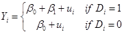. So this is just saying that Y has mean b₀ + b₁ in some cases and mean b₀ in other cases. So b₁ is interpreted as the difference in mean between the two groups (those with D=1 and those with D=0). Since it is the difference, it doesn't matter which group is specified as 1 and which is 0 – this just allows measurement of the difference between them.

Why do we always leave out a dummy variable? Multicollinearity. (See Chapter 6 of Stock & Watson.) If the intercept on the dummy is the difference in mean, then if we have 2 categories and 2 differences, then the regression is trying to figure out how these 2 categories are different from some 3^rd category (which is a null set) – so that gives an error.

Other 'tricks' of time trends (& functional form)

· If the X-variable is just a linear change [for example, (1,2,3,...25) or (1985, 1986,1987,...2010)] then regressing a Y variable on this is equivalent to taking out a linear trend: the errors are the deviations from this trend.

· The estimated coefficient β is the marginal change in Y for a change in X; if the Y-variable is a log function then the regression is interpreted as explaining percent deviations (since derivative of lnY = dY/Y, the percent change). (So what would a linear trend on a logarithmic form look like?)

· examine errors to check functional form – e.g. height as a function of age works well for age < 12 or 14 but then breaks down

· can get predicted Y values, , where both in-sample and out-of-sample

· plots of X vs. both Y and predicted-Y are useful, as are plots of X vs. error (note how to do these in SPSS – the dialog box for Linear Regression includes a button at the right that says "Save...", then click to save the unstandardized predicted values and unstandardized residuals).

In addition to the standard errors of the slope and intercept estimators, the regression line itself has a standard error.

Excel calculates OLS both as regression (from Data Analysis TookPak), as just the slope and intercept coefficients (formula values), and from within a chart

Nonlinear Regression

(more properly, How to Jam Nonlinearities into a Linear Regression)

· X, X², X³, … X^r

· ln(X), ln(Y), both ln(Y) & ln(X)

· dummy variables

· interactions of dummies

· interactions of dummy/continuous

· interactions of continuous variables

There are many examples of, and reasons for, nonlinearity. In fact we can think that the most general case is nonlinearity and a linear functional form is just a convenient simplification which is sometimes useful. But sometimes the simplification has a high price. For example, my kids believe that age and height are closely related – which is true for their sample (i.e. mostly kids of a young age, for whom there is a tight relationship, plus 2 parents who are aged and tall). If my sample were all children then that might be a decent simplification; if my sample were adults then that's lousy.

The usual justification for a linear regression is that, for any differentiable function, the Taylor Theorem delivers a linear function as being a close approximation – but this is only within a neighborhood. We need to work to get a good approximation.

Nonlinear terms

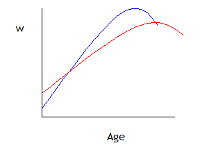
We can return to our regression using CPS data. First, we might want to ask why our regression is linear. This is mostly convenience, and we can easily add non-linear terms such as Age², if we think that the typical age/wage profile looks like this:

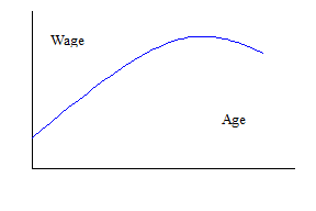
So the regression would be:

(where the term "..." indicates "other stuff" that should be in the regression).

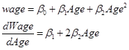
As we remember from calculus,

so that the extra “boost” in wage from another birthday might fall as the person gets older, and even turn negative if the estimate of (a bit of algebra can solve for the top of the hill by finding the Age that sets ).

We can add higher-order effects as well. Some labor econometricians argue for including Age³ and Age⁴ terms, which can trace out some complicated wage/age profiles. However we need to be careful of "overfitting" – adding more explanatory variables will never lower the R².

Logarithms

Similarly can specify X or Y as ln(X) and/or ln(Y). But we've got to be careful: remember from math (or theory of insurance from Intermediate Micro) that E[ln(Y)] IS NOT EQUAL TO ln(E[Y]) ! In cases where we're regressing on wages, this means that the log of the average wage is not equal to the average log wage.

(Try it. Go ahead, I'll wait.)

When both X and Y are measured in logs then the coefficients have an easy economic interpretation. Recall from calculus that with and , so -- our usual friend, the percent change. So in a regression where both X and Y are in logarithms, then is the elasticity of Y with respect to X.

Also, if Y is in logs and D is a dummy variable, then the coefficient on the dummy variable is just the percent change when D switches from zero to one.

So the choice of whether to specify Y as levels or logs is equivalent to asking whether dummy variables are better specified as having a constant level effect (i.e. women make $10,000 less than men) or having a percent change effect (women make 25% less than men). As usual there may be no general answer that one or the other is always right!

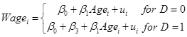
Recall our discussion of dummy variables, that take values of just 0 or 1, which we’ll represent as D_i. Since, unlike the continuous variable Age, D takes just two values, it represents a shift of the constant term. So the regression,

shows that people with D=0 have intercept of just b₀, while those with D=1 have intercept equal to b₀ + b₃. Graphically, this is:

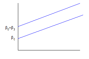
We need not assume that the b₃ term is positive – if it were negative, it would just shift the line downward. We do however assume that the rate at which age increases wages is the same for both genders – the lines are parallel.

The equation could be also written as

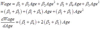
Dummy Variables Interacting with Other Explanatory Variables

The assumption about parallel lines with the same slopes can be modified by adding interaction terms: define a variable as the product of the dummy times age, so the regression is

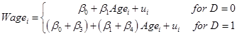
so that, for those with D=0, as before =b₁ but for those with D=1, . Graphically,

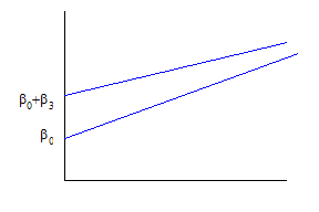
so now the intercepts and slopes are different.

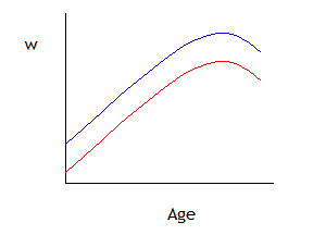
So we might wonder if men and women have a similar wage-age profile. We could fit a number of possible specifications that are variations of our basic model that wage depends on age and age-squared. The first possible variation is simply that:

which allows the wage profile lines to have different intercept-values but otherwise to be parallel (the same hump point where wages have their maximum value), as shown by this graph:

The next variation would be to allow the lines to have different slopes as well as different intercepts:

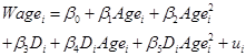
which allows the two groups to have different-shaped wage-age profiles, as in this graph:

(The wage-age profiles might intersect or they might not – it depends on the sample data.)

We can look at this alternately, that for those with D=0,

so the extreme value of Age (where ) is .

While for those with D=1,

so the extreme value of Age (where ) is . Or write the general value, for both cases, as where D is 0 or 1.

This specification, with a dummy variable multiplying each term: the constant and all the explanatory variables, is equivalent to running two separate regressions: one for men and one for women:

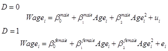
Where the new coefficients are related to the old by the identities: , , and . Sometimes breaking up the regressions is easier, if there are large datasets and many interactions.

Testing if All the New Variable Coefficients are Zero

You're wondering how to tell if all of these new interactions are worthwhile. Simple: Hypothesis Testing! There are various formulas, some more complicated, but for the case of homoskedasticity the formula is relatively simple.

Why any formula at all – why not look at the t-tests individually? Because the individual t-tests are asking if each individual coefficient is zero, not if it is zero and others as well are also zero. That would be a stronger test.

To measure how much a group of variables contributes to the regression, we look at the residual values – how much is still unexplained, after the various models? And since this is OLS, we look at the squared residuals. SPSS outputs the "Sum of Squares" for the Residuals in the box labeled "ANOVA". We compare the sum of squares from the two models and see how much it has gone down with the extra variables. A big decrease indicates that the new variables are doing good work. And how do we know, how big is "big"? Compare it to some given distribution, in this case the F distribution. Basically we look at the percent change in the sum of squares, so something like:

with the wavy equals sign to show that we're not quite done. Note that model 0 is the original model and model 1 is the model with the additional regressors, which will have a smaller residual (so this F can never be negative). To make this equal, we need to make it a bit like an elasticity – what is the percent change in the number of variables in the model? Suppose that we have N observations and that the original model has K variables, to which we're considering adding Q more observations. Then the original model has (N – K – 1) degrees of freedom [that "1" is for the constant term] while the new model has (N – K – Q – 1) degrees of freedom, so the difference is Q. So the percent change in degrees of freedom is . Then the full formula for the F test is

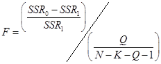Which is, admittedly, fugly. But we know its distribution, it's F with (Q, N-K-Q-1) degrees of freedom – the F-distribution has 2 sets of degrees of freedom. Calculate that F, then use Excel to calculate FDIST(F,Q,N-K-Q-1), which will output a p-value for the test. If the p-value is less than 5%, reject the null hypothesis.

Usually the formula is more complicated if, for example, we’re using heteroskedasticity-consistent errors. Usually you will have the computer spit out the results for you.

Multiple Dummy Variables

Multiple dummy variables, D_1,i , D_2,i , …,D_J,i, operate on the same basic principle. Of course we can then have many further interactions! Suppose we have dummies for education and immigrant status. The coefficient on education would tell us how the typical person (whether immigrant or native) fares, while the coefficient on immigrant would tell us how the typical immigrant (whatever her education) fares. An interaction of “more than Bachelor’s degree” with “Immigrant” would tell how the typical highly-educated immigrant would do beyond how the “typical immigrant” and “typical highly-educated” person would do (which might be different, for both ends of the education scale).

Many, Many Dummy Variables

Don't let the name fool you – you'd have to be a dummy not to use lots of dummy variables. For example regressions to explain people's wages might use dummy variables for the industry in which a person works. Regressions about financial data such as stock prices might include dummies for the days of the week and months of the year.

Dummies for industries are often denoted with labels like "two-digit" or "three-digit" or similar jargon. To understand this, you need to understand how the government classifies industries. A specific industry might get a 4-digit code where each digit makes a further more detailed classification. The first digit refers to the broad section of the economy, as goods pass from the first producers (farmers and miners, first digit zero) to manufacturers (1 in the first digit for non-durable manufacturers such as meat processing, 2 for durable manufacturing, 3 for higher-tech goods) to transportation, communications and utilities (4), to wholesale trade (5) then retail (6). The 7's begin with FIRE (Finance, Insurance, and Real Estate) then services in the later 7 and early 8 digits while the 9 is for governments. The second and third digits give more detail: e.g. 377 is for sawmills, 378 for plywood and engineered wood, 379 for prefabricated wood homes. Some data sets might give you 5-digit or even 6-digit information. These classifications date back to the 1930s and 1940s so some parts show their age: the ever-increasing number of computer parts go where plain "office supplies" used to be.

The CPS data distinguishes between "major industries" with 16 categories and "detailed industry" with about 50. Creating 50 dummy variables could be tiresome so I recommend that you use SPSS's syntax editor that makes cut-and-paste work easier. For example use the buttons to "compute" the first dummy variable then "Paste Syntax" to see the general form. Then copy-and-paste and change the number for the 51 variables:

COMPUTE d_ind1 = (a_dtind EQ 1).

COMPUTE d_ind2 = (a_dtind EQ 2).

COMPUTE d_ind3 = (a_dtind EQ 3).

COMPUTE d_ind4 = (a_dtind EQ 4).

COMPUTE d_ind5 = (a_dtind EQ 5).

COMPUTE d_ind6 = (a_dtind EQ 6).

COMPUTE d_ind7 = (a_dtind EQ 7).

You get the idea – take this up to 51. Then add them to your regression!

In other models such as predictions of sales, the specification might include a time trend (as discussed earlier) plus dummy variables for days of the week or months of the year, to represent the typical sales for, say, "a Monday in June".

If you're lazy like me, you might not want to do all of this mousework. (And if you really have a lot of variables, then you don't even have to be lazy.) There must be an easier way!

There is.

SPSS is a graphical interface that basically writes SPSS code, which is then submitted to the program. Clicking the buttons is writing computer code. Look again at this screen, where I've started coding the next dummy variable, ed_hs (from Transform\Compute Variables…)

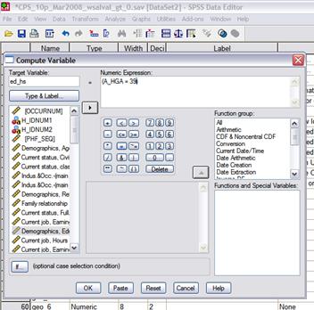
That little button, "Paste," can be a lot of help. It pastes the SPSS code that you just created with buttons into the SPSS Syntax Editor.

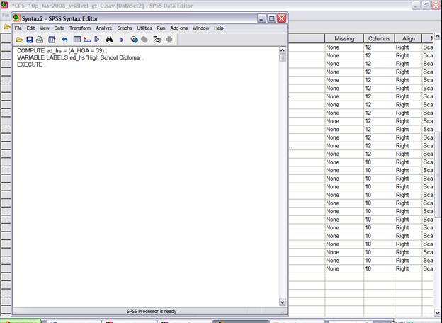
Why is this helpful? Because you can copy and paste these lines of code, if you are only going to make small changes to create a bunch of new variables. So, for example, the education dummies could be created with this code:

COMPUTE ed_hs = (A_HGA = 39) .

VARIABLE LABELS ed_hs 'High School Diploma' .

COMPUTE ed_smc = (A_HGA > 39) & (A_HGA < 43) .

VARIABLE LABELS ed_smc 'Some College' .

COMPUTE ed_coll = (A_HGA = 43) .

VARIABLE LABELS ed_coll 'College 4 Year Degree' .

COMPUTE ed_adv = (A_HGA > 43) .

VARIABLE LABELS ed_adv 'Advanced Degree' .

EXECUTE .

Then choose "Run\All" from the drop-down menus to have SPSS execute the code.

You can really see the time-saving element if, for example, you want to create dummies for geographical area. There is a code, GEDIV, that tells what section of the country the respondent lives in. Again these numbers have absolutely no inherent value, they're just codes from 1, New England, to 9, Pacific region. We can't put GEDIV into a regression but we can put geographic dummies. So we use the same procedure to create these:

COMPUTE geo_1 = (GEDIV = 1) .

COMPUTE geo_2 = (GEDIV = 2) .

COMPUTE geo_3 = (GEDIV = 3) .

COMPUTE geo_4 = (GEDIV = 4) .

COMPUTE geo_5 = (GEDIV = 5) .

COMPUTE geo_6 = (GEDIV = 6) .

COMPUTE geo_7 = (GEDIV = 7) .

COMPUTE geo_8 = (GEDIV = 8) .

COMPUTE geo_9 = (GEDIV = 9) .

EXECUTE.

You can begin to realize the time-saving capability here. Later we might create 50 detailed industry and 25 detailed occupation dummies.

If at some point you get stuck (maybe the "Run" returns errors) or if you don't know the syntax to create a variable, you can go back to the button-pushing dialogue box.

The final advantage is that, if you want to do the same commands on a different dataset (say, the March 2009) then as long as you have saved the syntax you can easily submit it again.

With enough dummy variables we can start to create some respectable regressions!

Use "Data\Select Cases…" to use only those with a non-zero wage. Then do a regression of wage on Age, race & ethnicity (create some dummy variables for these), educational attainment, and geographic region.

This starts to look as much like “writing code” as it would be, if you worked in R. Another reason to do stats work in R.

Why are we doing all of this? Because I want you to realize all of the choices that go into creating a regression or doing just about anything with data. There are a host of choices available to you. Some choices are rather conventional (for example, the education breakdown I used above) but you need to know the field in order to know what assumptions are common. Sometimes these commonplace assumptions conceal important information. You want to do enough experimentation to understand which of your choices are crucial to your results. Then you can begin to understand how people might analyze the exact same data but come to varying conclusions. If your results contradict someone else's, then you have to figure out what are the important assumptions that create the difference.