Class Oct 31

Happy ¡Dia de los Muertos!

Kevin R Foster, CCNY, ECO B2000

Fall 2013

I forgot to note last class, but this is great for learning about econometrics in R, http://cran.r-project.org/doc/contrib/Farnsworth-EconometricsInR.pdf

Panel Data

A panel of data contains repeated observations of a single economic unit over time. This might be a survey like the CPS where the same person is surveyed each month to investigate changes in their labor market status. There are medical panels that have given annual exams to the same people for decades. Publicly-traded firms that file their annual reports can provide a panel of data: revenue and sales for many years at many different firms. Sometimes data covers larger blocks such as states in the US or, if we're looking at macroeconomic development, even countries over time.

Other data sets are just cross-sectional, like the March CPS that we've used. If we put together a series of cross-sectional samples that don't follow the same people (so we use the March 2012, 2011, and 2010 CPS samples) then we have a pooled sample. A long stream of data on a single unit is a time series (for example US Industrial Production or the daily returns on a single stock).

In panel data we want to distinguish time from unit effects. Suppose that you are analyzing sales data for a large company's many stores. You want to figure out which stores are well-managed. You know that there are macro trends: some years are good and some are rough, so you don't want to indiscriminately reward everybody in good years (when they just got lucky) and punish them in bad years (when they got unlucky). There are also location effects: a store with a good location will get more traffic and sell more, regardless. So you might consider subtracting the average sales of a particular location away from current sales, to look at deviations from its usual. After doing this for all of the stores, you could subtract off the average deviation at a particular time, too, to account for year effects (if everyone outperforms their usual sales by 10% then it might just indicate a good economy). You would be left with a store's "unusual" sales – better or worse than what would have been predicted for a given store location in that given year.

A regression takes this even further to use all of our usual "prediction" variables in the list of X, and combine these with time and unit fixed effects.

Now the notation begins. Let the t-subscript index time; let j index the unit. So any observations of y and x must be at a particular date and unit; we have and then the k x-variables are each (the superscript for which of the x-variables). So the regression equation is

where (alpha) is the fixed effect for each unit j, (gamma) is the time effect, and then the error is unique to each unit at each time.

This is actually easy to implement, even though the notation might look formidable. Just create a dummy variable for each time period and another dummy for each unit and put the whole slew of dummies into the regression.

So, to take a tiny example, suppose you have 8 store locations over 10 years, 1999-2008. You have data on sales (Y) and advertising spending (X) and want to look at the relationship between this simple X and Y. So the data look like this:

X_1999,1	X_1999,2	X_1999,3	X_1999,4	X_1999,5	X_1999,6	X_1999,7	X_1999,8
X_2000,1	X_2000,2	X_2000,3	X_2000,4	X_2000,5	X_2000,6	X_2000,7	X_2000,8
X_2001,1	X_2001,2	X_2001,3	X_2001,4	X_2001,5	X_2001,6	X_2001,7	X_2001,8
X_2002,1	X_2002,2	X_2002,3	X_2002,4	X_2002,5	X_2002,6	X_2002,7	X_2002,8
X_2003,1	X_2003,2	X_2003,3	X_2003,4	X_2003,5	X_2003,6	X_2003,7	X_2003,8
X_2004,1	X_2004,2	X_2004,3	X_2004,4	X_2004,5	X_2004,6	X_2004,7	X_2004,8
X_2005,1	X_2005,2	X_2005,3	X_2005,4	X_2005,5	X_2005,6	X_2005,7	X_2005,8
X_2006,1	X_2006,2	X_2006,3	X_2006,4	X_2006,5	X_2006,6	X_2006,7	X_2006,8
X_2007,1	X_2007,2	X_2007,3	X_2007,4	X_2007,5	X_2007,6	X_2007,7	X_2007,8
X_2008,1	X_2008,2	X_2008,3	X_2008,4	X_2008,5	X_2008,6	X_2008,7	X_2008,8

and similarly for the Y-variables. To do the regression, create 9 time dummy variables: D2000, D2001, D2002, D2003, D2004, D2005, D2006, D2007, and D2008. Then create 7 unit dummies, D2, D3, D4, D5, D6, D7, and D8. Then regress the Y on X and these 16 dummy variables.

Then the interpretation of the coefficient on the X variable is the amount by which an increase in X, above its usual value for that unit and above the usual amount for a given year, would increase Y.

One drawback of this type of estimation is that it is not very useful for forecasting, either to try to figure out the sales at some new location or what will be sales overall next year – since we don't know either the new location's fixed effect (the coefficient on D9 or its alpha) or we don't know next year's dummy coefficient (on D2009 or its gamma).

We also cannot put in a variable that varies only on one dimension – for example, we can't add any other information about store location that doesn't vary over time, like its distance from the other stores or other location information. All of that variation is swept up in the firm-level fixed effect. Similarly we can't include macro data that doesn't vary across firm locations like US GDP since all of that variation is collected into the time dummies.

You can get much fancier; there is a whole econometric literature on panel data estimation methods. But simple fixed effects, put into the same OLS regression that we've become accustomed to, can actually get you far.

Multi-Level Modeling

After Fixed Effects and Random Effects, generalize from there. Multilevel Random Coefficient models (MRC) have layers. For example, if we use World Values Survey data and look at the satisfaction with financial situation, we can explain this in part by education levels. We will be interested in seeing how much variation there is within each of the education groups (how much difference in finances is there, among people with the same educational qualification?); then how much variation is there between the groups (how much difference is there, between the typical person with low education and the typical person with more education?).

Layer 1: explain Y as just varying for groups, so if there are groups j, j= 1, …, J, then:

So there is an overall intercept, β_0,0,and group intercepts, β_0,j. This is just like the dummy variable specification that we did before.

Instead of looking at the significance of dummy variable coefficients, we could approach it a different way. Ask, what is the correlation of people in the same group? If groups were assigned randomly without any information, we would expect this to be about zero. This is the Intraclass Correlation Coefficient, ICC. Just like with R², bigger is better although they’re graded on a curve so even as low as 0.05 might be sufficient.

Layer 2: Same structure as Layer 1 but on regression coefficients; so suppose that we had a dummy for gender, which had different effects by education, so

This is not quite as free-form as creating gender-education interactions, and letting those coefficients vary freely without restriction. Rather this assumes that the gender-education coefficients vary with some structure, usually that they are drawn from a normal distribution, with mean at the overall coefficient. Sometimes it is useful to impose a bit more structure on the problem.

Instrumental Variables

· Endogenous vs. Exogenous variables

o Exogenous variables are generated from "exo" outside of the model; endogenous are generated from "endo" within the model. Of course this neat binary distinction rarely is matched by the world; some variables are more endogenous than others

· Data can only demonstrate correlations – we need theory to get to causation. "Correlation does not imply causation." Roosters don't make the sun rise. Although Granger Causation from the logical inverse: not-correlate implies not-causation. If knowledge of variable X does not help predict Y, then X does not cause Y.

· In any regression, the variables on the right-hand side should be exogenous while the left-hand side should be endogenous, so X causes Y, . But we should always ask if it might be plausible for Y to cause X, , or for both X and Y to be caused by some external factor. If we have a circular chain of causation (so and ) then the OLS estimates are meaningless for describing causation.

· NEVER regress Price on a Quantity or vice versa!

Why never regress Price on Quantity? Wouldn't this give us a demand curve? Or, would it give us a supply curve? Why would we expect to see one and not the other?

In actuality, we don't observe either supply curves or demand curves. We only observe the values of price and quantity where the two intersect.

If both vary randomly then we will not observe a supply or a demand curve. We will just observe a cloud of random points.

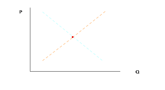
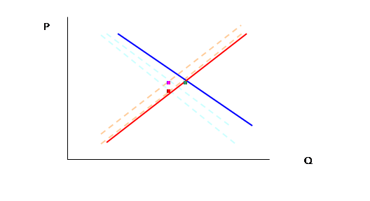
For example, theory says we see this:

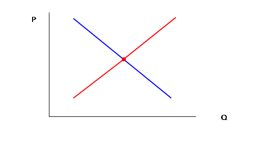
But in the world, we assume the dotted-lines and only actually observe the one intersection, the dot:

In the next time period, supply and demand shift randomly by a bit, so theory tells us that we now have:

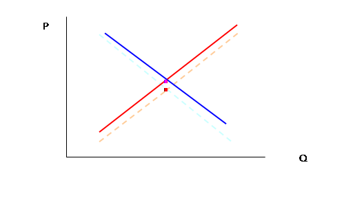
But again we actually now see just two points,

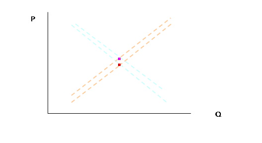
In the third period,

but again, in actuality just three points:

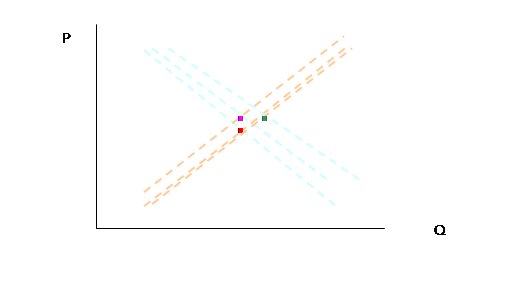
So if we tried to draw a regression line on these three points, we might convince ourselves that we had a supply curve. But do we, really? You should be able to re-draw the lines to show that we could have a down-sloping line, or a line with just about any other slope.

So even if we could wait until the end of time and see an infinite number of such points, we'd still never know anything about supply and demand. This is the problem of endogeneity. The regression is not identified – we could get more and more information but still never learn anything.

We could show this in an Excel sheet, too, which will allow a few more repetitions.

Recall that we can write a demand curve as P_d = A – BQ_d and a supply curve as P_s = C + DQ_s, where generally A, B, C, and D are all positive real numbers. In equilibrium P_d=P_s and Q_d=Q_s. For simplicity assume that A=10, C=0, and B=D=1. Without any randomness this would be a boring equation; solve to find 10 – Q = Q and Q*=5, P*=5. (You did this in Econ 101 when you were a baby!) If there were a bit of randomness then we could write and . Now the equilibrium conditions tell that and so and .

Plug this into Excel, assuming the two errors are normally distributed with mean zero and standard deviation of one, and find that the scatter looks like this (with 30 observations):

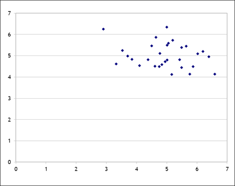
You can play with the spreadsheet, hit F9 to recalculate the errors, and see that there is no convergence, there is nothing to be learned.

On the other hand, what if the supply errors were smaller than the demand errors, for example by a factor of 4? Then we would see something like this:

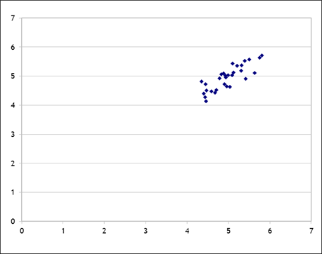
So now with the supply curve pinned down (relatively) we can begin to see it emerge as the demand curve varies.

But note the rather odd feature: variation in demand is what identifies the supply curve; variation in supply would likewise identify the demand curve. If some of that demand error were observed then that would help identify the supply curve, or vice versa. So sometimes in agricultural data we would use weather variation (that affects the supply of a commodity) to help identify demand.

If you want to get a bit crazier, experiment if the slope terms have errors as well (so and ).

Instrumental Variables Regression in R

There was a recent paper in the journal Economic Inquiry, by Cesur & Kelly (2013), "Who Pays the Bar Tab? Beer Consumption and Economic Growth in the United States," which concluded that beer consumption was bad for economic growth. I got data from the Brewer’s Almanac, provided online by the Beer Institute (beerinstitute.org) and the Bureau of Economic Analysis (bea.gov). This is not quite the same data that the paper used (less complete) but it gives a flavor (bad pun) of the results.

You can download the R data from InYourClass. Then run this regression,

regression1 <- lm(growth_rates ~ beer_pc + gdp_L + as.factor(st_fixedeff))

summary(regression1)

Where the growth rate of each state’s GDP is a function of per-capita beer consumption, a lag of state GDP (reflecting the general idea that poorer states might grow faster), as well as state fixed effects (each state has its own intercept). This shows a positive and statistically significant coefficient on per-capita beer consumption. So beer is good for growth?!

As Homer Simpson put it, "To alcohol! The cause of – and solution to – all of life's problems." That circularity of causation makes the statistics more complicated.

Richer people have more money to buy everything including beer, so economic growth might cause beer consumption. One way out, suggested by the article authors, is to use an instrument for beer consumption – the tax on beer. This is a plausible instrument since it likely causes changes in beer consumption (higher price, lower consumption, y’know the demand curve) but it unlikely to be affected by economic growth. So estimate an instrumental variables equation,

iv_reg1 <- lm(beer_pc ~ beertax)

summary(iv_reg1)

And see that indeed there is a negative coefficient (hooray for demand curves!) although it is certainly a weak instrument (R² less than 1%). Use the predicted value of beer consumption per capita as an instrument in the regression in place of the endogenous variable,

pred_beer <- predict(iv_reg1)

iv_reg2 <- lm(growth_rates ~ pred_beer + gdp_L + as.factor(st_fixedeff))

summary(iv_reg2)

To note that now beer consumption seems to have negative effects on economic growth (only significant at 10% level; the article adds some other variables to get it significant). I put some other variables in the dataset that you might play with – see if you can find the opposite result! (R code from a simple summary at http://www.r-bloggers.com/a-simple-instrumental-variables-problem/)

Finally note that you can use the AER package and ivreg() procedure for better results, since these estimated standard errors won’t be quite right – but that’s just fine-tuning.

The basic idea of instrumental variables is that if we have some regression,

But X and Y are endogenous, then suppose we had some variable Z, which is uncorrelated with Y but still explains X, then we can make a supplementary regression,

And get , the predicted values from that regression, then do the original regression as

Measuring Discrimination – Oaxaca Decompositions:

(much of this discussion is based on Chapter 10 of George Borjas' textbook on Labor Economics)

The regressions that we've been using measured the returns to education, age, and other factors upon the wage. If we classify people into different groups, distinguished by race, ethnicity, gender, age, or other categories, we can measure the difference in wages earned. There are many explanations but we want to determine how much is due to discrimination and how much due to different characteristics (chosen or given).

Consider a simple model where we examine the native/immigrant wage gap, and so measure , the average wages that natives get, and , the average wages that immigrants get. The simple measure, , of the wage gap, would not be adequate if natives and migrants differ in other ways, as well.

Consider the effect of age. Theory implies that people choose to migrate early in life, so we might expect to see age differences between the groups. And of course age influences the wage. If natives and immigrants had different average wages solely because of having different average ages, we would conclude very different reasons for this than if the two groups had identical ages but different wages.

For example, in a toy-sized 1000-observation subset of CPS March 2005 data, there are 406 natives and 77 immigrants workers with non-zero wages. The natives averaged wage/salary of $37,521 while the immigrants had $32,507. The average age of the natives was 39.5; the average age of the immigrants was 42.1. We want to know how much of the difference in wage can be explained by the difference in age.

Consider a simple model that posits different simple regressions for natives and immigrants:

We know that average wages for natives depend on average age of natives, :

and for immigrants as well, wages depend on immigrants' average age, :

The difference in average wages is:

but we can add and subtract the cross term, , to get:

Each term can be interpreted in different ways. The first difference, , is the difference in intercepts, the parallel shift of wages for all ages. The second, , is the difference in how the skills are rewarded: if everyone in the data were to have the same age, immigrants and natives would still have different wages due to these first two factors. The third is , which gives the difference in wage attributable only to differences in average age (even if those were rewarded equally). The first two are generally regarded as due to discrimination while the last is not.

The basic framework can be extended to other observable differences: in years of education, experience, or the host of other qualifications that affect people's wages and salaries.

From our discussions of regression models, we realize that the two equations above could be combined into a single framework. If we define an immigrant dummy variable as , which is equal to one if individual i is an immigrant and zero if that person is native born, we can write a regression model as:

where wages for natives depend on only and , while the immigrant coefficients are and . We construct and so the Oaxaca decomposition is now:

We note that unobserved differences in quality of skills can be measured as instead being due to discrimination. In our example, suppose that natives get a greater salary as they age due to the skills which they amass, but immigrants who have language difficulties learn new skills more slowly. In this case, older natives would earn more, increasing the returns to aging. This would be reflected as lower coefficients on age for immigrants than natives, and so evidence of discrimination. If we had information on English-language ability (SAT, TOEFL or GRE scores, maybe?), then the regression would show that a lack of those skills led to lower wages – no longer would it be measured as evidence of discrimination.

But this elides the question of how people gain the "skills" measured in the first place. If a degree from a foreign university gets less reward than a degree from an American university, is this entirely due to discrimination? What fraction of the wage differential arises from skill differences? In the US, African-American and Hispanic children tend to go to lower-quality schools (as measured by test scores or teacher qualifications). The lower subsequent wages might not be due to labor market discrimination (if firms rationally pay less for lower skills) but still be due to societal discrimination.

Consider the sort of dataset that we've been working with. Regressing Age, an Immigrant dummy, and an Age-Immigrant interaction on Wage provides the following coefficient estimates (for the same sub-sample as before):

where the immigrant dummy is actually positive (neither the immigrant dummy nor the immigrant-age interaction term are statistically significant, but I ignore that for now). With the average ages from above (natives 39.5 years old; immigrants 42.1), we calculate the gap in average predicted wages (natives are predicted to make an average wage of $37,561; immigrants to make $32,502) is $5058.08. The two first terms in the Oaxaca decomposition, relating to unexplained factors such as "discrimination" account for $5329.95, while the difference in age accounts for just -$271.86 (a negative amount) – this means that the ages actually imply that natives and immigrants ought to be closer in wages so they are even farther apart. We might reasonably believe that much of this difference reflects omitted factors (and could list out the important omitted factors); this is intended merely as an exercise.

Adding these additional variables is easy; I show the case for two variables but the model can be extended to as many variables as are of interest. Next consider a more complicated model, where now wages depend on Age and Education, so the two regressions for natives and immigrants are:

We know that average wages for natives depend on average age and education of natives, :

and for immigrants as well, wages depend on immigrants' average age, :

The difference in average wages is:

but we can add and subtract the cross terms , to get:

Again, the two terms showing the difference in average levels of external factors, and , are "explained" by the model while the other terms showing the difference in the coefficients are "unexplained" and could be considered as evidence of discrimination.

Exercises:

1. Do the above analysis on the current CPS data.

2. If instead you used log wages, but still kept just age as the measured variable, is your answer substantially different than in the previous question? (Note that the answers are in different units, so you have to think about how to convert the two answers.)

3. Consider other measures of skills, such as schooling and whatever other factors you consider important. How does this new regression change the Oaxaca decomposition?

4. What is the maximum fraction of wage difference that you can find (with different independent variables and regression specifications), related to discrimination? The minimum?

References:

Borjas, George (2003). Labor Economics.

Oaxaca, Ronald (1973). "Male-Female Wage Differentials in Urban Labor Markets," International Economic Review, 14(3).