Class Nov 7

Kevin R Foster, CCNY, ECO B2000

Fall 2013

Quantile Regression

If you recall our discussion of heteroskedasticity in things like the Age-Wage relationship, there is a well-known tendency for younger workers to have more compressed earnings, which then fan out as people get older.

For example, if we use the 2010 CPS data, we can look at people aged 25-55 who are working full time for most of the year and, even if we focus on a single educational group, for example those with a 4-year degree, we can see the spread here:

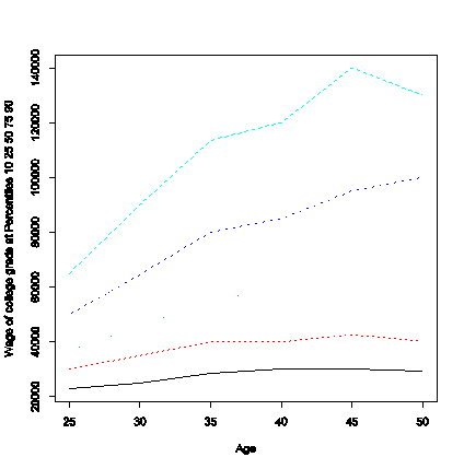
So the median worker saw a steady rise in wage: 30-yr-olds made just over $45,000 while 50-yr-olds made about $65,000; but those in the 25^th percentile went from $35,000 to $40,000 at age 30 and 50; those in the 75^th percentile went from $65,000 to $100,000.

One way to model these different results, for different percentiles, is with a quantile regression (mostly due to Roger Koenker), which uses a familiar regression framework to explain various percentiles.

In R this couldn’t be easier: just use the “quantreg” package and call the rq() function instead of lm(). (Note that it’s rq not qr; if you’ve done linear algebra you’ll recall the QR matrix decomposition.)

p_tiles <- c(0.1, 0.25, 0.5, 0.75, 0.9)

quantreg1 <- rq(WSAL_VAL ~ A_AGE + I(A_AGE^2) + female + afam + asian+ Amindian + Hispanic + immig + imm2gen + ed_hs + ed_collnd + ed_ASvoc + ed_ASacad + ed_coll + ed_adv + union + veteran, tau=p_tiles, data=data2)

summary(quantreg1)

plot(quantreg1)

Details are in the R file, lecturenotes9.R. This estimates age-wage profiles like this (again for those with a 4-year degree):

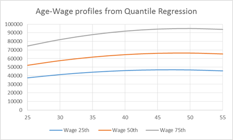
Which shows the spread.

Binary Dependent Variable Models

(Stock & Watson Chapter 9)

· Sometimes our dependent variable is continuous, like a measurement of a person's income; sometimes it is just a "yes" or "no" answer to a simple question. A "Yes/No" answer can be coded as just a 1 (for Yes) or a 0 (a zero for "no"). These zero/one variables are called dummy variables or binary variables. Sometimes the dependent variable can have a range of discrete values ("How many children do you have?" "Which train do you take to work?") – in this case we have a discrete variable. The binary and continuous variables can be seen as opposite ends of a spectrum.

· We want to explore models where our dependent variable takes on discrete values; we'll start with just binary variables. For example, we might want to ask what factors influence a person to go to college, to have health insurance, or to look for a job; to have a credit card or get a mortgage; what factors influence a firm to go bankrupt; etc.

· Linear Models such as OLS – NFG. These imply predicted values of Y that are greater than one or less than zero!

· Interpret our prediction of Y as being the probability that the Y variable will take a value of one. (Note: remember which value codes to one and which to zero – there is no necessary reason, for example, for us to code Y=1 if a person has health insurance; we could just as easily define Y=1 if a person is uninsured. The mathematics doesn't change but the interpretation does!)

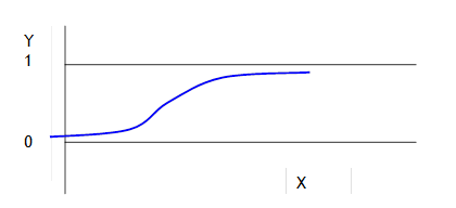
· want to somehow "bend" the predicted Y-value so that the prediction of Y never goes above 1 or below zero, something like:

· Probit Model

o where is the cdf of the standard normal

o is not constant

· Logit Model

o , where

o is not constant

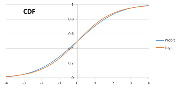
· differences (Excel sheet: probit_logit_compare.xls)

Clearly the differences are rather small; it is rare that we might have a serious theoretical justification for one specification rather than the other.

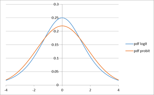
(Note that the logit function given above has standard error of so in the plots I scaled the probit by this factor).

· Measures of Fit

o no single measure is adequate; many have been proposed

o What probability should be used as "hit"? If the model says there is a 90% chance of Y=1, and it truly is equal to one, then that is reasonable to count as a correct prediction. But many measures use 50% as the cutoff. Tradeoff of false positives versus false negatives – loss function might well be asymmetric

Probit/Logit in SPSS

for logit: Analyze\Regression\Binary Logistic…

SPSS will generate lots of output; you can safely ignore just about everything in "Block 0" and concentrate on "Block 1". The last table shows "Variables in the equation" with columns for B, S.E., Wald, df, Sig., and Exp(B). The column for B is the estimate of the coefficient and S.E. is its standard error, same as always. But we don't estimate a t-stat but instead a Wald stat (a more complicated formula, don't worry) which combines with df to get a Sig. (a p-value). As usual, if the Sig. (p-value) is less than 0.05 then the variable is significant at the 5% level and you can make confident deductions from it. For now don't worry if you don't remember all of the details about the difference between t-tests and Wald tests from your stats classes. Just look at the calculated p-value to figure out which coefficients are significant. (Tests of multiple restrictions, which we did for the OLS model, are more complicated here so, again, don't worry about those now.)

for probit (Analyze\Regression\Probit…), SPSS wants the dependent variable (Response Frequency) and then Total Observed. For "Total Observed" just create a new variable that is always equal to 1 ("Transform\Compute" then create a new variable, ones, which always equals 1) and insert that variable. Leave "Factors" blank and insert the explanatory variables as "Covariate(s)"

SPSS calculates Probit with numerical iterations so it will sometimes return the message

Convergence Information

	Number of Iterations	Optimal Solution Found
PROBIT	20	No(a)

a Parameter estimates did not converge.

In this case, in the dialog box for "probit" usually you can choose the "Options… " button, then under "Criteria" increase the "maximum iterations" – as high as 999 if you have a small sample. The default number of iterations is just 20, which is often far too small! Sometimes, however, even 999 isn't enough. In that case, try a different program or a different set of variables. (Sometimes try the simple OLS version, which can at least catch some basic mistakes. Near-multicollinearity can kill you.)
After a successful estimation, SPSS will give you output like this:

Convergence Information

	Number of Iterations	Optimal Solution Found
PROBIT	26	Yes

The interpretation is analogous to OLS: the "Regression Coeff." is the coefficient on that variable, the "Standard Error" is its standard error, and the "Coeff./S.E." can be interpreted as a t-statistic. The remainder of the SPSS output can be safely ignored.

SPSS is generally lousy at logit/probit regressions of the type we're trying to do. It's just not designed for it.

Probit/Logit with R

For a logit estimation, just

regn_logit1 <- glm(Y ~ X1 + X2, family = binomial, data = data1)

for a probit estimation

regn_logit1 <- glm(Y ~ X1 + X2, family = binomial (link = 'probit'), data = data1)

Then the estimation results from “summary()” should be familiar.

Examples in lecturenotes9.R

Details of estimation
recall that OLS just gives a convenient formula for finding the values of 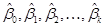that minimize the sum 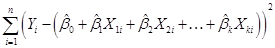. If we didn't know the formulas we could just have a computer pick values until it found the ones that made that squared term the smallest.
similarly a probit or logit coefficient estimates are finding the values of that minimize 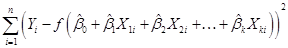, whether the function is a normal c.d.f. or a logit c.d.f.
Maximum Likelihood (ML) is a more sophisticated way to find these coefficient estimates – better than just guessing randomly.
For example the likelihood of any particular value from a normal distribution is the p.d.f., 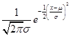. If we have 2 independent observations, from a distribution that is known to be normally distributed with variance of 1 (to keep the math easy) then the joint likelihood is 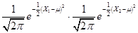. We want to find a value of µ that maximixes that function. This is an ugly function but we could note that any value of µ that maximizes the natural log of that function will also maximize the function itself (since is monotonic) so we take logs to get 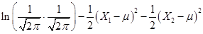. Take the derivative with respect to µ and set it equal to zero to get 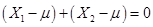so that . You should be able to see that starting with observations would get us 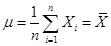so the average is also the maximum-likelihood estimator. A maximum-likelihood estimator could be similarly derived in cases where we don't know the variance (interestingly, that ML estimator of the standard error divides by n not (n – 1) so it is biased but consistent).
Maximizing the likelihood of the probit model is one or two steps more complicated but not different conceptually. Having a likelihood function with a first and second derivative makes finding a maximum much easier than the random hunt.

Properly Interpreting Coefficient Estimates:

Since the slope, , the change in probability per change in X-variable, is always changing, the simple coefficients of the linear model cannot be interpreted as the slope, as we did in the OLS model. (Just like when we added a squared term, the interpretation of the slope got more complicated.)

Return to the picture to make this much clearer:

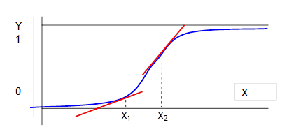
The slope at X₁ is rather low; the slope at X₂ is much steeper.

The effect of the coefficients now interacts with all of the other variables in the model: for example the effect of a person's gender on their probability of having health insurance will depend on other factors like their age and educational level. Women are generally less likely to have their own insurance than men, but how much less? Among young people with very low education, neither men nor women are very likely to be insured; among older people with very high education both are very likely insured. The biggest difference is toward the middle.

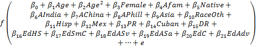
For example, very simple logit and probit estimations on the NHIS 2009 dataset (R program shows this in detail) gives the following coefficient estimates (I am suppressing notation on significance since it is not important here):

	Logit Estimate	Probit Estimate
(Intercept)	-1.519	-0.935
Age	0.059	0.036
Age-Squared	-0.0006	-0.0003
Female	-0.031	-0.017
African American	-0.576	-0.347
Native American Indian	-0.843	-0.503
Asian India	0.207	0.129
Asian Chinese	0.145	0.099
Asian Phillipines	0.162	0.095
Asian other	-0.181	-0.109
Race other	-0.323	-0.201
Hispanic	-0.607	-0.370
Mexican	0.097	0.057
Puerto Rican	0.123	0.077
Cuban	0.162	0.102
Dominican	-0.533	-0.320
Educ HS	0.744	0.455
Educ some college no degree	1.180	0.718
Educ AS vocational	1.186	0.725
Educ AS acad	1.501	0.911
Educ 4-yr degree	1.945	1.171
Educ Advanced degree	2.261	1.340
Immigrant	-0.717	-0.434
Married	0.501	0.304
Divorced/Widowed/Separated	-0.160	-0.092
Veteran	-0.443	-0.268
Region 2	-0.039	-0.023
Region 3	-0.391	-0.236
Region 4	-0.312	-0.189

The probability of having health insurance varies for different socioeconomic groups. We can interpret the signs in a straightforward way: the negative coefficients on the "female" variable indicate that women are less likely to have health insurance (not significant in either model though). African-Americans are less likely, along with Hispanics and Native Americans. Educational qualifications are positive and get larger.

But how large are these differences? For example, how much less likely to have health insurance are immigrants? It depends on the other variables. Intuitively, if a person is male, highly-educated, and married then he's probably insured (being an immigrant would them only slightly less so). So the change in probability associated with immigrant status would be low. At the opposite end, a woman without a high school diploma, who is single, is already be unlikely to be insured. Immigrant status hardly changes this. Only in the middle will there be a big effect.

We can calculate it straightforwardly, though.

Consider, say, a 35-yr-old non-immigrant African-American woman with an advanced degree, whose predicted probability of having health insurance is

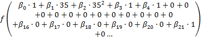
Summing the relevant coefficients (the intercept, female, and an advanced degree) gives a logit probability of

Which is 81.8%. For an otherwise-identical immigrant woman (also with an advanced degree) the probability is 0.687, so the change in probability is about 13.1 percentage points.

Comparing the probit estimates, we would just change the functional form and use the normal cdf instead of the logit function, so again from:

= (in R)

and find a probability for a non-immigrant woman as 0..812 and the immigrant woman to be 0.674, with a difference of 13.8 percentage points. These estimates from the logit and probit are very close.

Compare the change in probabilities for a married 50-yr-old white male with an advanced degree, who is either an immigrant or not. Now the probability of having insurance is, by the logit, 0.942 for the non-immigrant and 0.887 for the immigrant, a change of just 5.4 percentage points. From the probit the estimated probabilities are 0.951 for the non-immigrant and 0.889 for the immigrant, a change of 6.2 percentage points. This is because a married male with an advanced degree who is a union member is already highly likely to have health insurance, so the difference of being an immigrant or not makes half of the sized change compared with the previous example.

The details of this calculation are in an Excel spreadsheet, probit_logit_results.xls, that you can download.