About R
Econ B2000, Statistics and Introduction to Econometrics
Kevin R Foster, the City College of New York, CUNY
Fall 2014
R is a popular and widely-used statistical program. It might seem a bit overwhelming at first but you will learn to appreciate it. Its main advantage is that it is open-source so there are many 'packages' built by statisticians to run particular specialized estimations. BTW that means it's free for you to download and install – which is surely another advantage. [1]
Why learn this particular program? You should not be monolingual in statistical analysis, it is always useful to learn more programs. The simplest is Excel, which is very widely used but has a number of limitations – mainly that, in order to make it easy for ordinary people to use, they made it tough for power users. SPSS is the next step: a bit more powerful but also a bit more difficult. Next are Stata and SAS. Matlab is great but proprietary so not as widely used. Python might be important in some careers. The college has R, SPSS, SAS, and Matlab freely available in all of the computer labs. R is powerful, versatile, and widely used. This site has detailed analytics of which software is most common in job posts and other measures, http://r4stats.com/articles/popularity/ .
You might be tempted to just use Excel; resist! Excel doesn't do many of the more complex statistical analyses that we'll be learning later in the course. Make the investment to learn a better program; trust me on the cost/benefit ratio.
I will give a basic (albeit short) overview in these notes. If you want a deeper review, I included the book, A Beginner's Guide to R, by Zuur, Ieno and Meesters as a recommended text for the course as well as Applied Econometrics with R by Kleiber and Zeileis.
The Absolute Beginning
Start up R. On any of the computers in the Economics lab (6/150) double-click on the "R" logo on the desktop to start up the program. In other computer labs you might have to do a bit more hunting to find R (if there's no link on the desktop, then click the "Start" button in the lower left-hand corner, and look at the list of "Programs" to find R).
If you're going to install it on your home computer, download the program from R-project.org (http://www.r-project.org/) and follow those instructions – it has versions for Mac, Windows, and various Unix builds. You might want to also download R Studio (http://www.rstudio.com/) which is a helper program that sits on top of R to make it a bit friendlier to work with. (That's one of the advantages of R being open-source – the original developers didn't much worry about friendliness, so somebody else did.) Of course if you have trouble, Google can usually help.
With either R or R-Studio, you'll get an old-fashioned command line called "Console" (just " > ") where you can type in (or copy-and-paste in) commands to the program.
Until you get used to it, this might seem like a cost not a benefit. But consider if you've ever dug through someone else's Excel sheet (or even an old one of your own), trying to figure out, "how did they ever get that number?!?" For the sake of simplification and ease of use, it loses replicability. It can be tough to replicate what someone else did – but replication is the basis of science. So a little program that shows what you did each time can actually be really important. It also means you can use other people's code and instructions.
The guide, An Introduction to R, suggests these to give a basic flavor of what's done and hint at the power. Don't worry too much about each step for now, this is just a glimpse to show that with a few commands you can do some relatively sophisticated estimation – i.e. for a low cost you can get a large benefit.
x <- 1:20
w <- 1 + sqrt(x)/2
example1 <- data.frame(x=x,
y= x + rnorm(x)*w)
attach(example1)
This creates x and y variables (where the rnorm command creates random numbers from a normal distribution), puts them into a data frame, then attaches that data frame so that R can use it in later calculations. (What's a data frame? A way to collect together related data items.) Next some stats – create a linear model (that's the "lm") then a "lowess" nonparametric local regression, and plot the two estimations to compare. (Just copy and paste these, don't worry about understanding them for now!)
fm <- lm(y ~ x)
summary(fm)
lrf <- lowess(x,
y)
plot(x, y)
lines(x, lrf$y)
abline(0, 1, lty=3)
abline(coef(fm))
detach()
You should get a graph looking something like this (although with the random numbers, not exactly):
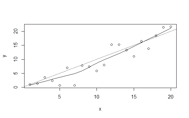
The final "detach" command just cleans up, it is the opposite of "attach".
For all of these commands, you can use R to type "help(__)" where you fill in __ in the obvious way to get help on commands including how to make various changes. Or shortcut with just "?__" so for example type "?summary" or "help(summary)". But as I said, don't worry much about those commands for now, I'm not expecting you to become an R-ninja overnight.
Basics in R
We will start with a few commands to get you able to follow along with these notes. For now you will use data that I've put together for you, ready to use in R, beginning with the Census Bureau's PUMS (Public Use Microdata Sample, from the American Community Survey, accessed from IPUMS). Download that data from InYourClass, the file is pums_NY.RData. I have restricted the sample to contain only people living in the state of New York. You might want to move that into a new directory (at least remember what directory you put it in), maybe name the new folder/directory " pums_NY." The commands are in the file, "working_on_PUMS.R" so you might download that too. (R is Case-Sensitive so careful with NY vs ny!)
Start with these commands in R or R-Studio; the first wipes the program clean:
rm(list = ls(all = TRUE))
setwd("C:\\ pums_NY")
# Change this as appropriate
load("pums_NY.RData")
The next, "setwd," is to set the working directory for this analysis. Your directory is somewhere on your computer, figure out the path name – in Windows it is usually something like setwd("C:\\Users\\Kevin\\Documents\\R\\pums_NY") and for Mac, setwd("~/desktop/R/pums_NY") – in both of those I'm assuming you created a folder called "R" and then inside that another folder, "pums_NY". The only difference is a doubled backslash in the name here in the program. As long as you had put the downloaded data into that directory and the program can find that directory, you should not have an error.
To check out the data use str(dat_pums_NY) which will show a list of the variables in the data and the first 10 or so lines of each variable, something like this
'data.frame': 196314 obs. of 57 variables:
$ Age : num 43 45 33 57 52 26 83 87 21 45 ...
$ female : num 1 0 0 0 1 0 1 0 0 0 ...
$ PERNUM : num 1 2 1 1 2 3 1 2 1 1 ...
(but longer!) In the next section I'll explain more about the data and what the lines mean but for now Age is the person's age in years and female is a logical 0/1 variable. So the first person is a 43-year-old female, next is a 45-year-old male, etc.
Next, run these
attach(dat_pums_NY)
NN_obs <- length(Age)
Which, as I said above, attaches the data frame to the program and then the next line should tell you how many people are in the data: 196,314.
Next we compare the average age of the men and the women in the data,
summary(Age[female
== 1])
summary(Age[!female])
The female dummy variable is a logical term, with a zero or one for false or true. The comparison is between those who have the variable female=1 (i.e. women) and those not female=1 (so logical not, denoted with the "!" symbol, i.e. men). I know, you can (and people do!) worry that this binary classification for gender misses some people; government statistics are just not there yet. I find this output,
Min. 1st Qu. Median Mean 3rd Qu. Max. 0.00 21.00 43.00 41.88 60.00 94.00 Min. 1st Qu. Median Mean 3rd Qu. Max. 0.00 19.00 39.00 39.19 57.00 94.00
So women are, on average, a bit older, with an average age of 41.9 compared with 39.2 for men. You might wonder (if you were to begin to think like a statistician) whether that is a big difference – hold onto that thought!
Alternately you can use
mean(Age[female
== 1])
sd(Age[female == 1])
mean(Age[!female])
sd(Age[!female])
to get mean and standard deviation of each. Later you might encounter cases where you want more complicated dummy variables and want to use logical relations "and" "or" "not" (the symbols "&", "|", "!") or the ">=" or multiplication or division.
As you're going along, if you're copying-and-pasting then you might not have had trouble, but if you're typing then you've probably realized that R is persnickety – the variable Age is not equivalent to a variable AGE nor age nor aGe …
Rather than cutting-and-pasting all of these command lines from the internet or your favorite word processing software, you might want something a bit easier. R-Studio has a text editor or you can find one online (I like Notepad + +) to download and install. Don't use MS Word, the autocorrect will kill you. But if you save the list of commands as a single file, you can just run the whole list all at once – which is easier once you get into more sophisticated stuff. As I mentioned above, I've saved them into a file called "working_on_PUMS.R" and you can create your own. That's also a help for when you say, "D'oh!" and realize you have to go back and re-do some work – if it's all in a file then that's easy to fix. (Feeling fancy, look into Sweave that combines the program with LATEX.)
Before you get too far, remember to save your work. The computers in the lab wipe the memory clean when you log off so back up your data. Either online (email it to yourself or upload to Google Drive or iCloud or InYourClass) or use a USB drive.
Codes of Variables
Some of the PUMS variables here have a natural interpretation, for instance Age is measured in years. Actually even this has a bit of a twist. If you type "hist(Age)" you'll get a histogram of Age, which doesn't show any problem. But if you do a somewhat more sophisticated graph (a nonparametric kernel density),
plot(density(Age[runif(NN_obs) < 0.1], bw = "sj"))
you can get a fancier picture, like this:

Note, for you geeks, that if you tried this with the
whole sample then the 200,000 observations would be too much, so I've randomly
selected 10% (that's the runif(NN_obs)<0.1 portion).
The kernel density is like a histogram with much smaller bins; in this case it shows a bit of weirdness particularly in the right, where it looks like there are suddenly a bunch of people who are 94 but nobody in between. This is due to a coding choice by the Census, where really old people are just labeled as "94". So if you were to get finicky (and every good statistician is!) you might go back to the calculations of averages previously and modify them all like this, mean(Age[(female == 1)&(Age<90)]) to select just those who are female and who are coded as having age less than 90. Also recall that this would not change the median values – which is one point in favor of that measure. You go do that, I'll wait right here…
Anyway, I was saying that many variables have a natural measure, like Age measured in years (below 90 anyway). Others are logical variables (called dummies) like female, Hispanic, or married – there is a yes/no answer that is coded 1/0. (Note that if you're creating these on your own it's good to give names that have that sort of yes/no answer, so a variable named 'female' is better than one named 'gender' where you'd have to remember who are 1 and who are 0.)
Other variables, like PUMA, have no natural explanation at all, you have to go to the codebook (or, in this case, the file pums_initial_recoding.r) to find out that this is "Public Use Microdata Area" where 3801 codes for Washington Heights/Inwood, 3802 is Hamilton Heights/Manhattanville/West Harlem, etc. The program will happily calculate the average value for PUMA (type in mean(PUMA) and see for yourself!) but this is a meaningless value – the average neighborhood code value? If you want to select just people living in a particular neighborhood then you'd have to look at the list below.
|
PUMA |
Neighborhood |
|
3701 |
NYC-Bronx CD 8--Riverdale, Fieldston
& Kingsbridge |
|
3702 |
NYC-Bronx CD 12--Wakefield, Williamsbridge
& Woodlawn |
|
3703 |
NYC-Bronx CD 10--Co-op City, Pelham Bay & Schuylerville |
|
3704 |
NYC-Bronx CD 11--Pelham Parkway, Morris Park & Laconia |
|
3705 |
NYC-Bronx CD 3 & 6--Belmont, Crotona Park East & East
Tremont |
|
3706 |
NYC-Bronx CD 7--Bedford Park, Fordham North & Norwood |
|
3707 |
NYC-Bronx CD 5--Morris Heights, Fordham South & Mount Hope |
|
3708 |
NYC-Bronx CD 4--Concourse, Highbridge
& Mount Eden |
|
3709 |
NYC-Bronx CD 9--Castle Hill, Clason
Point & Parkchester |
|
3710 |
NYC-Bronx CD 1 & 2--Hunts Point, Longwood & Melrose |
|
3801 |
NYC-Manhattan CD 12--Washington Heights, Inwood
& Marble Hill |
|
3802 |
NYC-Manhattan CD 9--Hamilton Heights, Manhattanville
& West Harlem |
|
3803 |
NYC-Manhattan CD 10--Central Harlem |
|
3804 |
NYC-Manhattan CD 11--East Harlem |
|
3805 |
NYC-Manhattan CD 8--Upper East Side |
|
3806 |
NYC-Manhattan CD 7--Upper West Side & West Side |
|
3807 |
NYC-Manhattan CD 4 & 5--Chelsea, Clinton & Midtown
Business District |
|
3808 |
NYC-Manhattan CD 6--Murray Hill, Gramercy & Stuyvesant Town |
|
3809 |
NYC-Manhattan CD 3--Chinatown & Lower East Side |
|
3810 |
NYC-Manhattan CD 1 & 2--Battery Park City, Greenwich Village
& Soho |
|
3901 |
NYC-Staten Island CD 3--Tottenville,
Great Kills & Annadale |
|
3902 |
NYC-Staten Island CD 2--New Springville & South Beach |
|
3903 |
NYC-Staten Island CD 1--Port Richmond, Stapleton & Mariner's
Harbor |
|
4001 |
NYC-Brooklyn CD 1--Greenpoint &
Williamsburg |
|
4002 |
NYC-Brooklyn CD 4—Bushwick |
|
4003 |
NYC-Brooklyn CD 3--Bedford-Stuyvesant |
|
4004 |
NYC-Brooklyn CD 2--Brooklyn Heights & Fort Greene |
|
4005 |
NYC-Brooklyn CD 6--Park Slope, Carroll Gardens & Red Hook |
|
4006 |
NYC-Brooklyn CD 8--Crown Heights North & Prospect Heights |
|
4007 |
NYC-Brooklyn CD 16--Brownsville & Ocean Hill |
|
4008 |
NYC-Brooklyn CD 5--East New York & Starrett
City |
|
4009 |
NYC-Brooklyn CD 18--Canarsie & Flatlands |
|
4010 |
NYC-Brooklyn CD 17--East Flatbush, Farragut & Rugby |
|
4011 |
NYC-Brooklyn CD 9--Crown Heights South, Prospect Lefferts & Wingate |
|
4012 |
NYC-Brooklyn CD 7--Sunset Park & Windsor Terrace |
|
4013 |
NYC-Brooklyn CD 10--Bay Ridge & Dyker
Heights |
|
4014 |
NYC-Brooklyn CD 12--Borough Park, Kensington & Ocean Parkway |
|
4015 |
NYC-Brooklyn CD 14--Flatbush & Midwood |
|
4016 |
NYC-Brooklyn CD 15--Sheepshead Bay, Gerritsen Beach & Homecrest |
|
4017 |
NYC-Brooklyn CD 11--Bensonhurst &
Bath Beach |
|
4018 |
NYC-Brooklyn CD 13--Brighton Beach & Coney Island |
|
4101 |
NYC-Queens CD 1--Astoria & Long Island City |
|
4102 |
NYC-Queens CD 3--Jackson Heights & North Corona |
|
4103 |
NYC-Queens CD 7--Flushing, Murray Hill & Whitestone |
|
4104 |
NYC-Queens CD 11--Bayside, Douglaston & Little Neck |
|
4105 |
NYC-Queens CD 13--Queens Village, Cambria Heights & Rosedale |
|
4106 |
NYC-Queens CD 8--Briarwood, Fresh Meadows & Hillcrest |
|
4107 |
NYC-Queens CD 4--Elmhurst & South Corona |
|
4108 |
NYC-Queens CD 6--Forest Hills & Rego
Park |
|
4109 |
NYC-Queens CD 2--Sunnyside & Woodside |
|
4110 |
NYC-Queens CD 5--Ridgewood, Glendale & Middle Village |
|
4111 |
NYC-Queens CD 9--Richmond Hill & Woodhaven |
|
4112 |
NYC-Queens CD 12--Jamaica, Hollis & St. Albans |
|
4113 |
NYC-Queens CD 10--Howard Beach & Ozone Park |
|
4114 |
NYC-Queens CD 14--Far Rockaway, Breezy Point & Broad Channel |
You could find the average age of women/men living in a particular neighborhood by adding in another "&" to the previous line so mean(Age[(female == 1)&(Age<94)&(PUMA == 4102)]) for Jackson Heights. (Or find the average age of each PUMA with tapply(Age, PUMA, mean) which, I admit, is a rather ugly bit of code.)
If you do a lot of analysis on a particular subgroup, it might be worthwhile to create a subset of that group, so that you don't have to always add on logical conditions. This can be done with the expressions:
restrict1
<- as.logical(Age >= 25)
dat_age_gt_25
<- subset(dat_pums_NY, restrict1)
So then you detach() the original dataset and instead attach(dat_age_gt_25). Then any subsequent analysis would be just done on that subset. Just remember that you've done this (again, this is a good reason to save the commands in a program) otherwise you'll wonder why you suddenly don't have any kids in the sample.
You might be tired and bored by these details, but note that there are actually important choices to be made here, even in simply defining variables. Take the fraught American category of "race". This data has a variable, RACED, showing how people chose to classify themselves, as 'White,' 'Black,' 'American Indian or Alaska Native,' (plus enormous detail of which tribe), Asian, various combinations, and many more codes.
Suppose you wanted to find out how many Asians are in a particular population. You could count how many people identify themselves as Asian only; you could count how many people identify as Asian in any combination. Sometimes the choice is irrelevant; sometimes it can skew the final results (e.g. the question in some areas, are there more blacks or more Hispanics?).
Again, there's no "right" way to do it because there's no science in this peculiar-but-popular concept of "race". People's conceptions of themselves are fuzzy and complicated; these measures are approximations.
Basics of government race/ethnicity classification
The US government asks questions about people's race and ethnicity. These categories are social constructs, which is a fancy way of pointing out that they are not based on hard science but on people's own views of themselves (influenced by how people think that other people think of them...). Currently the standard classification asks people separately about their "race" and "ethnicity" where people can pick labels from each category in any combination.
The "race" categories include: "White alone," "Black or African-American alone," "American Indian alone," "Alaska Native alone," "American Indian and Alaska Native tribes specified; or American Indian or Alaska native, not specified and no other race," "Asian alone," "Native Hawaiian and other Pacific Islander alone," "Some other race alone," or "Two or more major race groups." Then the supplemental race categories offer more detail.
These are a peculiar combination of very general (well over 40% of the world's population is "Asian") and very specific ("Alaska Native alone") representing a peculiar history of popular attitudes in the US. Only in the 2000 Census did they start to classify people in mixed races. If you were to go back to historical US Censuses from more than a century ago, you would find that the category "race" included separate entries for Irish and French and various other nationalities. Stephen J Gould has a fascinating book, The Mismeasure of Man, discussing how early scientific classifications of humans tried to "prove" which nationalities/races/groups were the smartest. Ta-Nehisi Coates says, "racism invented race in America."
Note that "Hispanic" is not "race" but rather ethnicity (includes various other labels such as Spanish, Latino, etc.). So a respondent could choose "Hispanic" and any race category – some choose "White," some choose "Black," some might be combined with any other of those complicated racial categories.
If you wanted to create a variable for those who report themselves as African-American and Hispanic, you'd use the expression (AfAm == 1) & (Hispanic == 1); sometimes stats report for non-Hispanic whites so (white == 1) & (Hispanic != 1). You can create your own classifications depending on what questions you're investigating.
The Census Bureau gives more information here, http://www.census.gov/newsroom/minority_links/minority_links.html
All of these racial categories make some people uneasy: is the government encouraging racism by recognizing these classifications? Some other governments choose not to collect race data. But that doesn't mean that there are no differences, only that the government doesn't choose to measure any of these differences. In the US, government agencies such as the Census and BLS don't generally collect data on religion.
Re-Coding complicated variables from initial data
If we want more combinations of variables then we create those. Usually a statistical analysis spends a lot of time doing this sort of housekeeping – dull but necessary.
Educational attainment is also classified with complicated codes: the original data has code 63 to mean high school diploma, 64 for a GED, 65 for less than a year of college, etc. I have transformed them into a series of dummy variables, zero/one variables for whether a person has no high school diploma, just a high school diploma, some college (but no degree), an associate's degree, a bachelor's degree, or an advanced degree. An advantage of these is that finding the mean of a zero/one variable gives the fraction of the sample who have a one. So if we wanted to find how many adults have various educational qualifications, we can use mean(educ_nohs[Age >= 25]) etc, to find that 14% have no high school, 28% have just a high school diploma, 16% have some college but no degree, 9% have an associate's, 18% have a bachelor's, and 15% have an advanced degree. You could do this by borough or neighborhood to figure out which places have the most/least educated people. (Ahem! You <cough> COULD do that right now. Or wait for the homework assignment.)
You can look at the variables in this dataset by the simple command str(dat_pums_NY) which gives the name of each variable along with the first few data points of each. (I did this a few sections ago, so this is review.) For this data it will show
$ Age : num 43 45 33 57 52 26 83 87 21 45 ... $ female : num 1 0 0 0 1 0 1 0 0 0 ... $ PERNUM : num 1 2 1 1 2 3 1 2 1 1 ...
so the first person in the data is aged 43 and is female. PERNUM is the Person Number in the household, so each new value of 1 indicates a new household. So the first household has the 43-year-old female and a 45-year-old male, then the second household has just a 33-y-o male, etc. You should look over the other variables in the data; the end of the file has some of the codes – for example the Ancestry 1 and 2 variables have enormously detailed codings of how people state their ancestry.
How to install packages
R depends crucially on "packages" – that's the whole reason that the open-source works. Some statistician invents a cool new technique, then writes up the code in R and makes it available. If you used a commercial package you'd have to wait a decade for them to update it; in R it's here now. Also if somebody hacks a nicer or easier way to do stuff, they write it up.
Some of the programs I use will depend on R packages. Installing them is a 2-step process: first, from R Studio, choose "Tools \ Install Packages" from the menu (from plain R, it's "Packages \ Install Packages"). Then in the command line or program, type library(packagename). (Fill in name of package for "packagename".)
Time Series in R
This next part is mostly optional, just again showing some of the stuff that R can easily do for time series data. First install some packages (for each package, use install.package("zoo") and so forth)
library(zoo)
library(lattice)
library(latticeExtra)
library(gdata)
rm(list = ls(all = TRUE))
Then get data from online – also a cool easy thing to do with R.
#
original data from:
oilspot_url <-
"http://www.eia.gov/dnav/pet/xls/PET_PRI_SPT_S1_D.xls"
oilspot_dat <- read.xls(oilspot_url,
sheet = 2, pattern = "Cushing")
oilfut_url <-
"http://www.eia.gov/dnav/pet/xls/PET_PRI_FUT_S1_D.xls"
oilfut_dat <- read.xls(oilfut_url,
sheet = 2, pattern = "Cushing, OK Crude Oil Future Contract 1")
Use R's built-in system for converting jumbles of letters and numbers into dates,
date_spot <- as.Date(oilspot_dat$Date, format='%b %d%Y')
date_fut <- as.Date(oilfut_dat$Date,
format='%b %d%Y')
Then R's "ts" for time-series and the "zoo" package.
wti_spot <- ts(oilspot_dat$Cushing..OK.WTI.Spot.Price.FOB..Dollars.per.Barrel.,
start = c(1986,2), frequency = 365)
wti_fut1
<-
ts(oilfut_dat$Cushing..OK.Crude.Oil.Future.Contract.1..Dollars.per.Barrel.,
start = c(1983,89), frequency = 365)
wti_sp_dat <- zoo(wti_spot,date_spot)
wti_ft_dat <- zoo(wti_fut1,date_fut)
wti_spotfut <- merge(wti_sp_dat,wti_ft_dat,
all=FALSE)
And plot the results.
plot(wti_spotfut, plot.type =
"single", col = c("black", "blue"))
#
tough to see any difference, so try this
wti_2013
<- window(wti_spotfut, start = as.Date("2013-01-01"),
end = as.Date("2013-12-31"))
plot(wti_2013,
plot.type = "single", col =
c("black", "blue"))
#
if you like this publication, you can get fancier...
asTheEconomist(xyplot(wti_2013, xlab="Cushing WTI Spot Future Price",))
De-bugging
Without a doubt, programming is tough. In R or with any other program, it is frustrating and complicated and difficult to do it the first few times. Some days it feels like a continuous battle just to do the simplest thing! Keep going despite that, keep working on it.
Your study group will be very helpful of course.
There are lots of online resources for learning R; like R for Beginners by Paradis, or the main intro from the R website, An Introduction to R.
I mentioned some books at the beginning, A Beginner's Guide to R, by Zuur, Ieno and Meesters and Applied Econometrics with R by Kleiber and Zeileis.
Then there are all of the websites, including:
· http://flowingdata.com/2012/06/04/resources-for-getting-started-with-r/
· http://statmaster.sdu.dk/bent/courses/ST501-2011/Rcard.pdf with lists of common commands
· http://www.cookbook-r.com/ a "cookbook" for R
· http://www.statmethods.net/ with "Quick R"
If you have troubles that you can't solve, email me for help. But try to narrow down your question: if you run 20 lines of code that produce an error, is there a way to reproduce the error after just 5 lines? What if you did the same command on much simpler data, would it still cause an error? Sending emails like "I have a problem with errors" might be cathartic but is not actually useful to anyone. If you've isolated the error and read the help documentation on that command, then you're on your way to solving the problem on your own.