|
Lecture Notes 11,Value at Risk VAR K Foster, CCNY, Spring 2010 |
|
|
Learning Outcomes (from CFA exam)
Students will be able to:
· discuss the advantages and limitations of VAR as a measurement of risk to a portfolio.
from
Value at Risk is one of the basic measures of the risk of a loss in a particular portfolio. It is typically stated in a form like, "there is a one percent chance that, over a particular day of trading, the position could lose" some dollar amount. We can state it more generally as VaR(X,N) = V, where V is the dollar amount of the possible loss, X is the percentage (managers might commonly be interested in the 1%, 5%, or 10%), and N is the time period (one day, one week, one month). To get from one-day VaR to N-day VaR, if the risks are independent and identically distributed, we multiply by .
Or, in one irreverent definition, VaR is "a number invented by purveyors of panaceas for pecuniary peril intended to mislead senior management and regulators into false confidence that market risk is adequately understood and controlled" (Schachter, from gloriamundi.org).
VaR is called upon for a variety of tasks (enumerated in Duffie & Pan 1997):
measure risk exposure; ensure correct capital allocation; provide information to counterparties, regulators, auditors, and other stakeholders; evaluate and provide incentives to profit centers within the firm; and protect against financial distress. Note that the final desired outcome (protection against loss) is not the only desired outcome. Being too safe costs money and loses business!
VaR is an important component of bank regulation: the Basel Accord sets capital based on the 10-day 1% VaR (so, if risks are iid, then the 10-day Var is times larger than the one-day). The capital is set at least 3 times as high as the 10-day 1% VaR, and can be as much as four times higher if the bank's own VaR calculations have performed poorly in the past year. If a bank hits their own 1% VaR more than 3 times in a year (of 250 trading days) then their capital adequacy rating is increased for the next year. Poor modeling can carry a high cost!
If we graph the distribution of possible returns of a portfolio, we can interpret VaR as a measure of a percentile. If we plot the cumulative distribution function (cdf) of the portfolio value, then the VaR is simply the inverse of the probability, X:

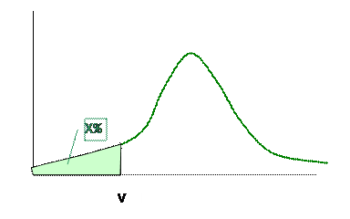
Or if we graph the probability density function (pdf), then V is the value that gives a particular area under the curve:

This is obviously similar to hypothesis testing in statistics.
Typically we are concerned with the lower tail of losses; therefore some people might refer to either the 1% VaR or the 99% VaR. From the mathematical description above, the 99% VaR would seem to be the upper tail probability (therefore the loss in a short position) but this is rarely the intent – the formulation typically refers to the idea that 99% of losses will be smaller (in absolute value) than V.
Basel rules for bank solvency divides assets into "banking book" that is not often traded and "trading book" that is. Trading book risk measured by 10-day 99% VAR; capital must be multiple of that.
There are three basic methods of computing the Value at Risk of some portfolio:
· parametric models that assume some error distribution,
· historical returns that use a selection of past data, and
·
computationally intensive
Each of these typically has two steps: first determine a possible path for the value of some underlying asset, then determine the change in the value of the portfolio assets due to it.
The parametric model case assumes that future returns can be
modeled with some statistical distribution such as the
An extension of the parametric approach is to use the Greeks that we have derived from the Black-Scholes-Merton model (under the assumption of normally-distributed errors) to calculate possible changes in the portfolio values.
We can also incorporate information from options prices into the calculation of forward Value at Risk. For instance, if S&P 500 option prices imply a high VIX (volatility) then the model could use this volatility instead of the historical average. In extracting information from derivatives prices we must be careful of the difference between the risk-neutral distribution and the distribution of actual price changes – VaR is based on actual changes not some perfectly-hedged portfolio!
The basic method of historical returns would just select some reference period of history (say, the past 2 years), order the returns from that period, and select the X% worst one to represent the Value at Risk based on past trading history. Basically instead of using some parametric cdf, this method uses a historical cdf (an empirical cdf). The choice of historical period means that this method is not quite as simple as it might sound.
Each method has strengths and weaknesses. The parametric method is quick and easy to implement with a minimum of computing power. It is good for calculating day-to-day trading swings for thickly-traded assets and conventional derivatives (plain vanilla or with well-specified Greeks). But most common probability distributions were developed for making inferences about behavior in the center of the probability mass – means and medians. The tails tend to be poorly specified and so do not perform as well.
These are for single assets; many assets are held as hedges where the value of one asset is expected to change as the value of another asset changes – they are not independent random variables but are correlated – they covary. For example we often refer to a stock's beta, telling how it is believed to covary with market aggregate returns.
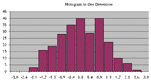
Each method must choose which underlying variables are considered and which covariances. The covariances are tough (particularly for historical simulations) since the "curse of dimensionality" quickly takes hold. For example, consider a histogram of 250 observations (one trading year) of returns on a single variable:

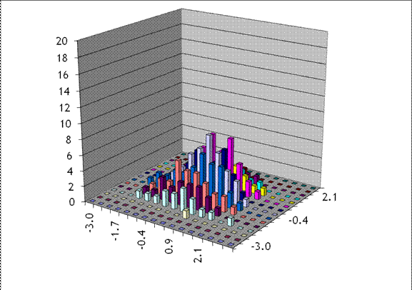
with the distribution of the same 250 observations but now incorporating the joint behavior of two variables:

You can see that now many of the boxes represent a single observation (they are just 1 unit high) while the maximum value is 8 (down from 40 previously). A series of "historical simulations" that drew from these observations would have very few options, compared with a parametric draw that needs only the correlation between the variables and a specification of a distributional form. The imposition of a normal distribution might be unrealistic but it might be less bad than the alternatives.
To handle the dimensionality problem, we might use Principal Components Analysis, that breaks down complex movements of variables (like the yield curve) into simpler orthogonal "factor" movements that can then be used in place of the real changes.
For interest rates, could use the simplest duration definition, that , so the percent change in a bond price, when the interest rate shifts by some amount, is given by the duration. But this is usually too simplistic so use cash flow mapping.
Sometimes use a Quadratic Model for portfolio value – not just linear but second-order terms. This uses information on option gammas – remember those? So, for example, a long call might have a low probability of expiring in the money but a higher probability of expiring without value – the pdf of its returns has the right-hand tail stretched farther out – a positive gamma. A long put has negative gamma – it's pdf of returns is stretched out leftward.
So a Quadratic Model adds a term. Instead of just modeling the change in portfolio value, , as , we use . For multiple assets we need to define a "cross gamma" term.
To consider the VaR constructions in more detail, consider how to define the VaR for a portfolio with just a single asset. If this asset has a normal distribution then a parametric VaR would say there is a 1% chance that a day's trading will end more than -2.326 standard deviations below average (see the example above for details on calculating V from a Z statistic). We would use information on the past performance of the asset to determine its average and standard deviation. A historical simulation VaR would rank, say, the past 4 years of data (approximately 1000 observations) to find the worst 10.
There is a general tradeoff between the amount of historical data used and the degree of imposed inference. No model is completely theory-independent (the historical simulation model assumes that the future will be sampled from some defined past). As the amount of theory increases, more inferences can be drawn but at a cost: if the theory is incorrect then the inferences will be worse (although if the theory is right then the inferences will be sharper).
All these methods share a weakness of looking to the past for guidance, rather than seriously considering future events that are genuinely new. Stress Testing tries to push them further, by asking how a portfolio position would react to extreme price/volume changes.
Back Testing acts to check out that the percentages seem to line up. Not only must the number of actual "hits" be close to the predicted number, but they should also be independent of each other. "Hits" that are clustered indicate that the VaR is not adequately dependent upon current market valuations. Back testing can also explore the adequacy of other percentile measures of VaR, on the insight that, if the 5% VaR (or 10%, or 0.5%, or whatever) is wrong then we might have more skepticism for the validity of the 1% measure.
All of these methods also find only a single percentile of the distribution. Suppose a firm has some exotic option which will be worth $100 in 99.5% of the trading days but will lose $1000 on 0.5%. Then the 1% VaR is $100; it's not very risky by standard VaR measures. Even if the option lost $10,000 or $1,000,000 or even enough to put the firm bankrupt, on 0.5% of trading days, the calculated VaR would not change! Now ½ of 1% doesn't seem large but there are 250 trading days in the typical year so that almost guarantees that such an outcome would happen. In the pictures of the cdf and pdf above, this is simply that the left-hand tail can be drawn out to stretch into huge losses. Therefore some advocate the calculation of a Conditional VaR, which is the expected loss conditional on it being among the worst 1% of trading days.
The VaR methods all basically assume that the trading desk is a machine that can generate any basket of risk/return on the efficient frontier that is desired; the role of management is to specify how much risk they want to take on (and therefore how high of a return they want). This assumes that risk is a univariate measure with a defined specification, but there are many sources of risk. If management is genuinely so disconnected from the trading desk that is taking on this risk, then there is a real problem that no VaR can solve! If management is more closely involved, then they should understand the panoply of risks.
As a simple example, remember the housing crisis. Before 2007, many analysts reassured themselves and their clients that a geographically diverse portfolio of mortgages could be less risky. Why? Because those mortgage-backed securities would only lose value if a lot of people had mortgage problems all at once. If we think of 1000 people paying mortgages, facing random risks so that some fraction run into trouble (but this fraction is not correlated!) then the bundling of mortgages makes it safer – like life insurance. Now of course we know that housing markets aren't quite that way, there are regular cycles in certain geographic areas. When a local economy booms, its real estate does too; and vice versa. That suggests that geographic diversity would help. Indeed one mantra, repeated over and over, was that the U.S. had not seen a country-wide decrease in real estate values since the Great Depression – which was true enough. Many mortgage-backed securities were safe as long as the country didn't have a monster recession, of a size unseen since the 1930s – but was that safe enough? There were other problems, too – again, of a degree not widely seen or understood in advance but clear in hindsight. Many bundles of mortgages were not diverse in the type of borrower – so "subprime" mortgages or "NINJA" mortgages would be all bundled together. These would lose value if many of the mortgages underlying them went into default. The statistic about overall U.S. property values was invoked again – but now with even less justification. A more clear-eyed risk assessment would ask if there were historical episodes when the riskiest and weakest borrowers had all gone to default together. Tough to answer, since many of these mortgage products were brand-new. Without bundling, nobody would have previously given a loan of several hundred thousand dollars to a NINJA – somebody who couldn't/wouldn't even provide documentation that they had a job or any income!
VaRs are a single tool of risk management not a silver bullet. Emanuel Derman writes that risk managers "need to love markets and know what to worry about: bad marks, mis-specified contracts, uncertainty, risk, value-at-risk, illiquid positions, exotic options" (in Risk, May 2004). VaR is just one part of a risk manager's toolkit, although its presentational charm and simplicity of communication can make it seductive.
Why does it break down? How did it work in the Financial Crisis? Read the NYTimes article by Joe Nocera. One quote describes how VaR came to be used within companies:
For instance, during his early years as a risk manager, pre-VaR, Guldimann often confronted the problem of what to do when a trader had reached his trading limit but believed he should be given more capital to play out his hand. “How would I know if he should get the increase?” Guldimann says. “All I could do is ask around. Is he a good guy? Does he know what he’s doing? It was ridiculous. Once we converted all the limits to VaR limits, we could compare. You could look at the profits the guy made and compare it to his VaR. If the guy who asked for a higher limit was making more money with lower VaR” — that is, with less risk — “it was a good basis to give him the money.”