|
Lecture Notes 2, Bonds (Ch 4) and Hedging (Ch 3) K Foster, CCNY, Spring 2010 |
|
|
Learning Outcomes (from CFA exam)
Students will be able to:
§ interpret interest rates as required rate of return, discount rate, or opportunity cost;
§ calculate and interpret the effective annual rate, given the stated annual interest rate and the frequency of compounding;
§ solve time value of money problems when compounding periods are other than annual;
§ calculate and interpret the future value (FV) and present value (PV) of a single sum of money, an ordinary annuity, an annuity due, a perpetuity (PV only), and a series of unequal cash flows;
§ draw a time line and solve time value of money applications (for example, mortgages and savings for college tuition or retirement).
§ describe the characteristics and calculate the gain/loss of forward rate agreements (FRAs);
§ calculate and interpret the payoff of an FRA, and explain each of the component terms;
§ define European option, American option, and the concept of moneyness of an option;
§ differentiate between exchange-traded options and over-the-counter options;
§ define intrinsic value and time value and explain their relationship;
|
|
|
On using these Lecture Notes:
We sometimes don't realize the real reason why our good habits work. In the case of taking notes during lecture, this is probably the case. You're not taking notes in order to have some information later. If you took your day's notes, ripped them into shreds, and threw them away, you would still learn the material much better than if you hadn't taken notes.
The process of listening, asking "what are the important things said?," answering this, then writing out the answer in your own words that's what's important!
So even though I give out lecture notes, don't stop taking notes during class. Take notes on podcasts and video lectures, too. Notes are not just a way to capture the fleeting sounds of the knowledge that the instructor said, before the information vanishes. Instead they are a way for your brain to process the information in a more thorough and more profound way. So keep on taking notes, even if it seems ridiculous. The reason for note-taking is to take in the material, put it into your own words, and output it. That's learning. |
|
|
From
Remember basic definitions: a "basis point" is one-hundredth of a percentage point. So if the Fed cut rates by one half of one percent (say, from 4.25% to 3.75%) then this is a cut of 50 basis points (bp, sometimes pronounced "bip") from 425 bp to 375 bp. Ordinary folks with, say, $1000 in their savings accounts don't see much of a change (50 bp less means $5) but if you're a major institution with $100m at short rates then that can get into serious money: $500,000.
A dollar today is not worth a dollar in the future, even without any inflation. Remember that the true cost of something is its opportunity cost: what must be given up in order to get it. To get a dollar in one year I don't need to give up a dollar today, not when I can put about 97 cents into the bank and, with 3% interest, get $1 in a year's time.
There are 2 basic issues that we must address: the rate of compounding and the fact that interest rates change over time.
Rate of Compounding
We often use
continuously-compounded interest, so that an amount invested at a fixed
interest rate grows exponentially.
Unless you've read the really fine print at the bottom of some loan
document, you probably haven't given much thought to the differences between
the various sorts of compounding annual, semi-annual, etc. Do that now:
|
If $1 is invested and grows at rate R then |
annual compounding means I'll have |
(1 + R) after one year. |
|
If $1 is invested and grows at rate R then |
semi-annual compounding means I'll have |
|
|
" |
compounding 3 times means I'll have |
|
|
… |
… |
… |
|
" |
compounding m times means I'll have |
|
|
" |
… |
… |
|
" |
continuous compounding (i.e. letting |
eR after one year. |
This odd irrational
transcendental number, e, was first used by John Napier and William Outred in
the early 1600's; Jacob Bernoulli derived it; Euler popularized it. It is or
. It is the expected minimum number of uniform
[0,1] draws needed to sum to more than 1.
The area under
from 1 to e is equal to 1.
Sometimes we write eR; sometimes exp{R} if the stuff buried in the superscript is important enough to get the full font size.
Since interest was being paid in financial markets long before the mathematicians figured out natural logarithms (and computing power is so recent), many financial transactions are still made in convoluted ways.
For an interest rate is 5%, this quick Excel calculation shows how the discount factors change as the number of periods per year (m) goes to infinity:
|
m per year |
(1+R/m)^m |
Discount Factor |
|
1 |
1.05 |
0.952380952 |
|
2 |
1.050625 |
0.951814396 |
|
4 |
1.0509453 |
0.951524275 |
|
12 |
1.0511619 |
0.951328242 |
|
250 |
1.0512658 |
0.95123418 |
|
360 |
1.0512674 |
0.951232727 |
|
|
|
|
|
infinite |
1.0512711 |
0.951229425 |
So going from 12 intervals (months) per year to 250 intervals (business days) makes a difference of one basis point; from 250 to an infinite number (continuous discounting) differs by less than a tenth of a bp.
A bond should be worth the present discounted value of its cash flows. Actually any financial instrument (if the flows are known with certainty) ought to be, which is why we want to work out the discounting on simple bonds before getting to more complicated payoffs.
What is present discounted value (PDV)?
Recall that we first determine the schedule of cash flows and then discount those back to the present. The schedule of cash flows can be most easily represented as a timeline, so for example payments of $100 in 3 months, $200 in 6 months, and $300 in 9 months, then a payment of $5000 in 12 months, would be represented as:
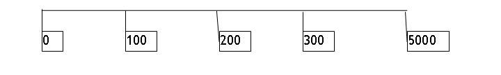
But we need to be precise about the units. The $100 in 3 months is not 100 of today-dollars but 100 of today-plus-3-months-dollars. You might not usually make a precise distinction but, for a large institution, the difference is important. Cash has an opportunity cost. So we could write the present discounted value as:
$T=.25 100 + $T=.5 200 + $T=.75 300 + $T=1 5000.
(Note that time is measured
in years so 3 months is of a year.)
But adding different units
gives us a meaningless result we need to get these values into common
units. We want to find some ratio (a
discount factor) that gives
for each future date, T.
So the PDV would be
calculated as these cash flows times some function that accounts for the time
delay. Of course we can't have just time
economics says that just a quantity is never
enough, we need a price too! What is the price of time? Sounds like a deep philosophical issue but
economists answer "interest rate."
So we include the quantity
(time) and its price (the interest rate) into a function which we will (for
now) label PDV(T,r). This function gives
the ratio, .
So the PDV of the bond with the timeline shown above is
We measure T in years so we can then substitute in for the different values, getting:
What is the function,
PDV(T,r)? It can take one of two basic
forms, depending on whether we are considering continuous time or discrete time
periods. In continuous time ,
sometimes written as exp{-rT} so that we don't need to squint at the
superscript. We'll assume continuous
time for a while here.
This would be simple if the interest rate, r, were constant over the entire time period. We will start with that simple case but we want to work up to the more complicated version. So for the example above, if the interest rates are unchanging over the next 12 months then r.25 = r.5 = r.75 = r1 = r and this function is:
= 100 e-.25r + 200 e-.5r + 300
e-.75r + 5000 e-r
If r = 0.06 (a 6% interest
rate) then we can easily calculate this value using a table in Excel.
|
A |
B |
C |
D |
E |
|
|
T= |
r= |
discount
factor |
cash flow |
discounted
cash flow |
|
|
0.25 |
0.06 |
0.985112 |
100 |
98.511194 |
|
|
0.5 |
0.06 |
0.970446 |
200 |
194.08911 |
|
|
0.75 |
0.06 |
0.955997 |
300 |
286.79924 |
|
|
1 |
0.06 |
0.941765 |
5000 |
4708.8227 |
|
|
|
|
|
|
|
|
|
|
|
|
|
5288.2222 |
sum of
discounted cash flows |
First set a column that
gives the T to use at each date when there is cash flow (column A). Then figure out what interest rate applies
for cash discounted from that date (column B), and the cash flow on that date
(column D). Then the discount factor (in
continuous time) is exp(-rt) (column C).
The discounted cash flow is the product of the discount factor and the
cash flow (column E); then the sum of the discounted cash flows is the present
discounted value.
Changing Interest Rates over Time
If the interest rate
changes over the period, then we have to account for the changing interest
rates. How do we do this? We have to distinguish between two types of
interest rates: those measuring the rate from today until some date in the
future ("zero rate") and those measuring the rate from some date in
the future to some date even farther into the future (forward rates). The zero rate can be thought of as the
average of all of the forward rates.
If we graph the evolution
of the interest rate then we might have a graph like this:
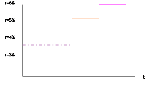
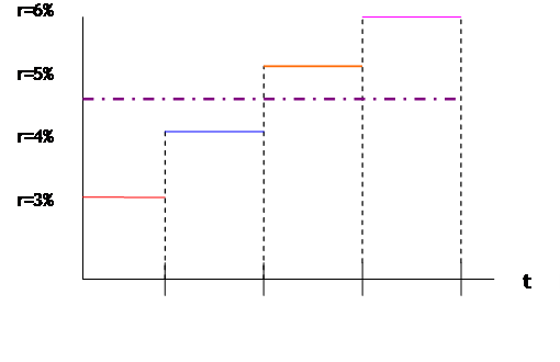
where the interest rate
over the first quarter is 3% and then the interest rate over the second quarter
(from the first quarter to the second quarter) is 4%. The zero rate for the first-and-second
quarters is 3.5%, the average, which is the dot-dash line in the picture. If the interest rate in the third quarter
rises to 5% then the zero rate for the first-second-and-third quarters (the
3-quarter zero rate) is 4%, which is the average of 3, 4, and 5 percent:
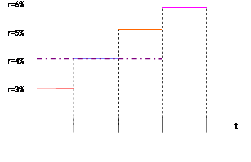
Then, finally, if the
interest rate during the fourth quarter is 6%, the one-year zero rate is 4.5%,
which is the average of 3, 4, 5, and 6.
If interest rates for the
first quarter are 4% and the forward rate for the second quarter is 6%, then
the forward rate over the third quarter is 3% and the forward rate over the
fourth quarter is 5%, then the average rate is 4.5% -- this would be the rate
over the whole year (the one year zero rate).
If we are interpolating
rates over different periods then we need to worry about weighted
averages. Suppose that we have one forward
rate going from T1 to T2, which we call RF. The zero rate over T1 is R1. To find the zero rate over T2,
just take the weighted average, so that
so that
or, equivalently,
.
To find a forward rate from
the zero rates, the formula is .
In the language of micro,
the forward rate is the marginal rate, which changes the zero rate.
If the path of the interest
rate is more complicated then the formulas can get more complicated (each
interest rate would be multiplied by a weight representing the fraction of the
time period during which the interest rate had that value). [In an
extreme case where the interest rate is continuous then we would integrate,
Rieman-style, over the intervals.] The instantaneous
forward rate at time T is .
Generally for bond pricing,
we want to use the zero rate for the appropriate time period in each PDV( )
function.
Forward Rate Agreement (FRA) is
where company trades a fixed rate (for some future period of time) against the
actual rate that occurs in that future period.
If the one-year rate is 5% and the 2-year rate is 5.5%, then that means
that the forward rate (from one to two years out) is 6%. Suppose that I don't have money to invest
today, but I expect to have it in one year, so I can't buy a 2-year bond but I
still want to lock-in that 6% rate. The
FRA solves this problem. Define RK
as the agreed forward rate, RM as the actual market rate, L is the
principal amount, and the time goes from T1 to T2. Then one company gets L(RK RM)(T1
T2) and the other gets the
negative.
Often theory tells us to
use a "risk-free" interest rate in valuing some financial asset. In the US, securities issued by the Federal
government, such as T-bills and Treasury bonds are generally defined as
risk-free; but traders commonly use LIBOR 1-mo, 3-mo, 6-mo, 12-mo. This is from the Euro-currency market (often
cited as "Eurodollar" market, even though it's not necessarily in its continued existence is a reminder of how
technology allows disintermediation of regulators!).
If you remember your
money-and-banking class, monetary policy is typically made by the Fed using
Repos (repurchase agreements) often overnight.
Let's go back to the
example of the stream of cash flows:
But now with the interest
rate changing (along the path that we showed in the graph above), so we need to
find the zero rates. The one-quarter
zero rate is 3%. The second quarter
forward rate is 4% so the zero rate is 3.5%.
The third quarter forward rate is 5% and the three quarter zero rate is
4%. Finally the fourth quarter forward
rate is 6% so the one-year zero rate is 4.5%.
So we substitute these values into the equation:
then use the continuous-time PDV function of
exp{ } to get:
.
To again create a table we
just change the values of the zero interest rate over each time period:
|
T= |
r= |
discount
factor |
cash flow |
discounted
cash flow |
|
|
0.25 |
0.03 |
0.992528 |
100 |
$
99.25 |
|
|
0.5 |
0.035 |
0.982652 |
200 |
$
196.53 |
|
|
0.75 |
0.4 |
0.740818 |
300 |
$
222.25 |
|
|
1 |
0.045 |
0.955997 |
5000 |
$4,779.99 |
|
|
|
|
|
|
|
|
|
|
|
|
|
$5,298.02 |
sum of
discounted cash flows |
So the steps required to
calculate the present discounted value are:
1.
figure out at
what time every amount of cash flows in or out,
2.
figure out
whether the compounding is to be done continuously or over discrete time,
3.
figure out the
zero rate for each of the relevant times when cash flows,
4.
calculate the
discount factors
5.
multiply the
cash times the discount factor to get the discounted cash flow
6.
sum the
discounted cash flows.
The formula would be
,
where ci is the
cash flow at date i, ri is the zero rate to that time period, and ti
is the time (expressed in fractions of one year) and B is the price of the
bond.
Certain types of cash flows
are discounted using continuous-time compounding while other sorts of cash
flows are discounted at discrete intervals.
You can think of these schedule differences as just different units of
measurement, like Celsius and Fahrenheit.
Discrete Compounding
Sometimes we work in
discrete time units, so the interest paid to $1 at rate R, if compounded m
times, is . So the discounted value of a dollar after 1
year is
(note the negative sign in the exponent) and
the discounted value after T years is
. So if we are compounding at discrete
intervals, m, then we have PDV(r,t,m) =
and we can consider PDV(r,t,∞) as exp(-rt) a
limiting case.
So to take the example
above, with
$T=.25
100 + $T=.5 200 + $T=.75 300 + $T=1 5000.
worth
=
then we put in this
different PDV function. So if we put
this into Excel, if the interest rate were constant and m=0.5 (semi-annual
compounding) then the bond is worth:
|
t |
r |
m |
PDV |
cash |
discounted cash value |
|
0.25 |
0.06 |
0.5 |
0.998302 |
100 |
99.8302 |
|
0.5 |
0.06 |
0.5 |
0.996606 |
200 |
199.3212 |
|
0.75 |
0.06 |
0.5 |
0.994913 |
300 |
298.4740 |
|
1 |
0.06 |
0.5 |
0.993223 |
5000 |
4966.1167 |
|
|
|
|
|
|
|
|
|
|
|
|
|
5563.7420 |
The difference in valuation
is not small, from 5564 to 5298, so you might ask why such a difference? Which one is right? The answer is that it depends on your
opportunity cost which valuation more accurately characterizes
your next-best use of the funds?
(Alternately we rely on past precedent: certain bonds are typically
valued in certain ways, so that's how we do it.)
Going Backwards
Having worked out how to
value a bond from a given set of interest rates, then we can invert the function
and ask how to find interest rates from bond prices. This is the more typical case: bonds are
traded but interest rates are not usually directly traded. A bond that pays a fixed schedule of money
has a present discounted value which is its price. If we don't know what interest rates were
used to get the market price of the bond, then we have to work backwards from the present discounted value back to the
interest rates that were used for the discounting.
The simplest case is a bond
that pays zero coupons but only makes a single repayment. For instance if a bond makes a single payment
of 7000 in one year then the present discounted value is the market price. If we assume that there is discrete
compounding only once per year then the market price, P, is 7000/(1+r). If we knew r then we could find the valuation
of the bond; if we know the market price then we know the implied interest
rate. This rate is the bond yield, the interest rate that
makes the bond valuation equal to its price.
In the simple example above, where P = 7000/(1+r), we can see the
inverse relationship between interest rates and bond prices. When rates rise, bond prices fall and vice
versa. If instead it were continuously
compounded then P=7000e-r.
Again you can see the inverse relationship.
Bonds typically are issued
at some notional "par value" (sometimes the "face value")
which is the notional amount that the interest is computed from. For instance a bond might have a par value of
1000 and pay 50 per year forever this is a five percent par yield. But as interest
rates change subsequent to the bond's issuance, its market price will also
change and the par value will become just a relic of history.
The bond yield gets more complicated as the number of cashflow dates
rises since we are trying to make more inferences. If we have a bond that, say, returns $3000
after 1 year and $4000 after 2 years then with simple annual compounding the
value is 3000/(1+r1) + 4000/(1+r2)2. If we have only the market price then we can
make no further progress we have a single equation with two
unknowns. If we know either of the zero
rates (or if we know that the interest rate remained constant, or some other
relationship between r1 and r2) then we can solve for the
implied bond yield.
Bond yield
is the single constant discount rate, applied to the actual coupon payments,
that makes the bond price equal to its market price. (If there were no coupon payments, then this
is just the zero rate that gives the current bond price.)
Par yield
is the coupon rate that causes the bond price to equal its par value (the
principal).
Examples:
Find the present discounted
value of $1000 paid in six months, if the 7% interest rate is compounded
continuously.
= 1000 * PDV(0.5, 0.07) = 1000 e-.5*.07 =
1000 * 0.965605 = $965.61
We can, of course, work
backwards as well. If the market values
a bond, that pays $1000 in six months, at $965.61, then what continuous-time
interest rate is implied?
Now we set 965.61 = 1000 * PDV(0.5,r) = 1000 e-.5r
so 0.96561 = e-.5r and ln(0.96561) = 0.5r so that r = 0.06999, which
is 7% with a bit of rounding error.
|
|
Now do the same exercise
if interest is semi-annual, quarterly, or monthly. We have = 1000 * PDV(0.5, 0.07,m) where m=2, 4, or 12. which is
For m=2, this is
1000/(1.035) =966.18; for m=4 this is 965.90; for m=12 this is 965.70. |
The remainder is steadily
working up new details.
Now to find the present
discounted value of $1000 paid in 6 months and in 12 months, if the interest rate
is still constant at 7% compounded continuously, this is 1000 * PDV(0.5, 0.07)
+ 1000 * PDV(1, 0.07) = 1000 e-.5*.07 + 1000 e-1*.07 =
965.604 + 932.39 = 1898.
Working backwards again, if
the market values this bond at 1898 then what interest rate is implied? Again, set 1898 = 1000 * PDV(0.5, r) + 1000 *
PDV(1, r) = 1000 e-.5r + 1000 e-1r. Now
we have to remember the rules of exponents: we can't just add the two terms
together (just like x2 + x3 ≠ x5!). So we can use a computer to figure out which
values of r give the correct bond value.
You could experiment with some different values to figure out that,
indeed (what a shock!) r = 0.07 does, indeed, work. It's a numerical problem; there is no general
analytic solution.
Note that the interest rate
used for discounting has absolutely nothing to do with the par yield! A bond might be sold with a $100,000 face
value paying $5000 annually, implying a 5% par yield. But if interest rates rise then that bond
isn't worth as much (& vice versa) the "5%" isn't relevant in any way
once the bond has been issued.
Next with interest rates
changing over time. So the rate for
three months forward is different from the rate six months forward, because the
rate for 3-6 months ahead is different.
Consider two bonds that pay
a quarterly coupon and, so, we use quarterly compounding to find their present
value. One bond, with face value of
$100,000, pays its final quarterly coupon ($1200) in one quarter as well as the
100,000 of principal. The other bond
pays a quarterly coupon in one quarter and then, 2 quarters from today, makes
its last quarterly payment and its par value.
From the market prices of those two bonds, find the implied zero rates
for one quarter and for two quarters, as well as the second quarter forward
rate. If the market gives a price for
the shorter-term bond of $100,074.17 and a price for the 2-quarter bond of
$99,903.31 then we have two equations:
$100,074.17
= and
$99,903.31
= .
To solve, we would first
calculate the bond yield implied for the first bond to get r1 =
0.045 = 4.5%. Then once we have r1
we can substitute into the second equation and find that r2 =
0.05. So the forward rate over the
second quarter must be 5.5% (enough of a rise to get the average of 4.5% and
5.5% up to the 5% zero rate).
If the same question were
posed but with continuous compounding then the precise value of the interest
rate would change. Now we would have two
equations that:
$100,074.17
= (100000+1200)exp(-.25r1) and
$99,903.31
= 1200 exp(-.25r1) + (100000+1200) exp(-.5r2).
Again these equations can
be solved one at a time, knitting up the solutions from the first equation on there is no reason we couldn't do this for
every quarter for the next 30 years! (That sounds like a good exam question, doesn't it? I'm joking, of course, 30 years is too many…)
This method would work just
as well if the first bond made no payments for a year (so it paid 101200 after
5 quarters) while the second bond made a payment of 1200 in 5 quarters and then
101200 in 6 quarters. The discount
factor would be larger but the basic solution strategy would be the same.
All of these interest rates
are part of the yield curve, which shows the interest rates over different time
horizons. This set of zero rates
(derived from bond prices) is then useful for discounting other cash flows.
For some bonds there may
not be enough quoted prices to figure out every step of the yield curve so
analysts would have various methods for filling in the holes.
Once we get accustomed to
using interest rates to figure out bond prices, we want to then find a quick
rule that avoids the complicated math (it's tough to figure e to decimal powers
or natural logs in your head!). This is duration it approximates the percentage change in a
bond price for a given change in the interest rate; so
.
Duration is the time at which the cashflows are paid, with the weighting as
just the present discounted value of the cashflow, so
.
If duration is in discrete
time then we replace the exp{ } function with the appropriate PDV function and
the term is called modified duration.
The rate at which duration
changes, as the interest rate changes, is convexity
(it is the second derivative with respect to changes in the interest rate).
Don't worry about the formula for now but later, if you do a fixed-income securities
class or need it for your job, you can remember that you've heard of it.
Recall payoff graphs, nets
to positions including call/put.
Chapter 3
concentrates on hedgers.
A hedge is basically
locking in cash flows at an early date before the asset changes hands. Consider a position, St, that will
have value ST at some future date, T. If that asset is hedged then a forward is
sold at time T and bought at time t, so that the net asset position is ST
FT + Ft. We expect that, by the time of expiration,
the spot and futures price will be equal (or else there would be arbitrage
opportunities) so we expect that, by date T, ST
FT = 0. So the hedge is exchanging a volatile price
(St becoming ST) for a known price, Ft.
Short Hedge:
own an asset and short a forward to sell at a pre-specified price.
examples: gold mines might sell the gold, that's
still in the ground, at pre-determined prices at some date in the future to
"lock in" a profit; farmer can sell the crop forward; exporter with
short-term receivables might pre-sell (sell forward) to lock in a profit rate. Consider an insurer selling annuities in
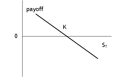
Payoff Graphs: a short
forward position at strike price K pays off as:
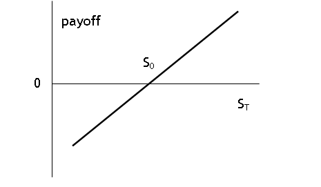
While a long spot position
(at S0) pays off as:
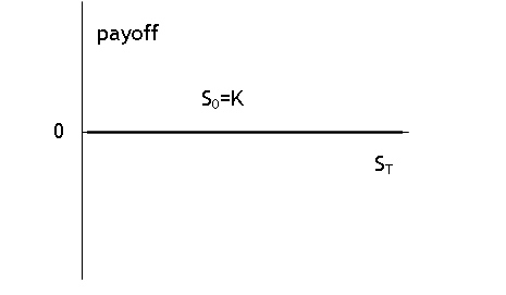
So if S0 = K
then when we add together the two payoff graphs then the net payoff to the
portfolio (of one long spot position plus one short forward) is zero
everywhere:
If the price at which the
initial asset was bought (S0) is not the same as the forward price (K)
then the net payoff is a bit more complicated:
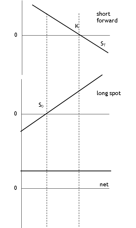
To find the net position
graphically, just line up the two graphs of the base positions, find a
convenient point (where one or the other is zero) and add. Then move right or left, figuring out how
much one payoff increases and the other payoff decreases (if there is a hedge).
So could do others: if
K<S0, for non-hedge positions (both long or both short).
Hedge can be considered by
comparing the money lost on the asset position with the money gained from the
offsetting hedge. For instance, if the
insurer above is getting ¥100,000,000 in 3 months. Right now the rate is 90¥/$ so this is worth
$1,111,111 (=100m/90). If the rate
increases to 95¥/$ then this is worth only $1,052,632. The movement of ¥5 in the FX rate meant a
loss of $58,480 on the asset position.
If the forward price is also 90¥/$ then selling ¥90 forward (getting one
dollar delivered in 3 months) would mean that, if the yen increased to 95 per
dollar then the short forward position would mean that the company could sell
¥90 for $1 and still have ¥5 left over to buy dollars (0.0526 worth). This 5-penny gain is small compared to the
$58,480 loss but the company could sell more than ¥90. How many 90¥/$ contracts? 58,480/0.0526 =1,111,111 worth (which is
exactly the number we discovered earlier).
This might seem like the long way to go about it but it is worth showing
the basic method: one position loses a certain amount; it can be hedged if I
can find some other position that would gain that same amount. Most companies use hedges with much more
complicated structures, but the basic idea remains: construct two offsetting
positions so that, as one loses the other gains (and vice versa).
Long Hedge:
will buy an asset in the future and buy a forward to but at a pre-specified
price.
examples: manufacturers that use mining products
(gold, copper, etc) or plastics can buy in advance and lock-in their
costs. Southwest Airlines made huge
profits, compared with some of their competitors, when they bought fuel forward
for mid 2008 before the oil price rose drastically. Their competitors had to pay higher prices
while Southwest reaped the profits.
(Their competitors, of course, noted that by 2009, when fuel prices had fallen,
then Southwest was paying extra for insurance.)
A long forward pays off as

Can work an example in
reverse (as above): how to hedge a short position today with a long forward.
Plenty of individuals
hedge, even though they might not realize it.
Property owners choosing mortgages must choose between fixed-rate (where
the interest rate paid is constant for the life of the loan) or variable or
varieties in-between (sometimes a rate is fixed for a few years at first and then
varies more often). A business, that
employs a person at a fixed salary even though the employee's productivity
might vary, is, in some way, hedging.
Most insurance companies pass along risks through re-insurance, which
are then shared among a wide net of different financial companies.
Why do so many companies
hedge? Wouldn't their investors want
exposure to certain risks? For instance
investors might buy shares in both Exxon/Mobile (that does well when oil prices
rise) as well as Ford (which does worse as oil prices rise). If both companies hedge their positions, then
that risk-diversification is lost. (An
investor would have to buy shares in the counter-parties.) Insurers take a hit from hurricanes (like
Katrina) but many pass along the risks as they hedge their positions (there are
catastrophe bonds that are linked to occurrences of natural disasters).
But the reality is that
many companies forecast their earnings, go through a great deal of effort to
communicate this "guidance" to the analysts following their shares,
and they know that their share price falls when they don't meet expectations;
it's difficult to communicate the many sources of risk that might be faced by a
global company with revenues in many different currencies and costs paid for
many different goods. Even internally, a
company might want to sort out whether a particular division made money by luck
(a favorable FX move) or skill (even after hedging they still out-performed). A hedge means that the company can set its
benchmarks and make profits only in its particular areas of comparative
advantage. Return to the example of the
gold mine: by selling forward they commit that they will make profit if they
are efficient at extracting gold; they will lose money if they are not efficient
at that. Random fluctuations in gold
prices will not drive their results; their profits instead come only from their
own efficiency.
Competitive pressures can
also be important and so every industry (even every firm) must make decisions
based on their own particular needs.
Finally, these hedges might
allow a company to spread the risk more broadly to willing investors. An individual company might hedge in order to
pass the risk on to the global financial markets. Instead of a small number of companies losing
a lot of money, a large number of investors around the world can each lose a
small amount.
Most hedging is not perfect
the real world is messier. Basis
= St
Ft.
If the asset that is held and the futures contract are the same then at
expiration the Basis should be zero. So
if the position is opened at time t and closed out at time T, then we would
like ST=FT. Define
bt = St
Ft and bT = ST
FT.
Then if the company has assets St, it could choose not to
hedge, in which case it would have ST at the end of the period. If it hedges then it would still get the
return of ST at the end but would then accrue profits to the forward
positions, Ft
FT, so the net position would be [this is the same formula as at the
beginning, just with a slightly different interpretation]
ST
+ Ft FT = Ft + bT.
If it is a perfect hedge
then the basis is zero at time T and the value is known at time t; if the basis
is not zero then there is residual risk basis
risk. This is generally common when
the asset position is not one of the standard contracts traded on
exchanges.
This basis risk could have
many sources: perhaps a local oil company would like to hedge its costs. Heating oil is traded on NYMEX but the price
paid by an oil company (at its local delivery) is not quite the same as the
NYMEX price (delivered to NY harbor). Or
sales are not known exactly so the company hedges a substantial fraction of its
anticipated sales (but not all). Or a
company hedges individual stock holdings (on a company with a high beta) with,
say, S&P500 index futures (to save trading costs). Or a company's bonds could be hedged with
forward Treasuries and options on the company stock.
If we consider a
distinction between St (the asset held) and St* (the
asset that is traded on a market) then the position will be ST FT + Ft. If we add and subtract ST* then we
can rearrange that to get Ft + (ST* - FT) + (ST
ST*)
the first term in parentheses is the basis
risk between the "ideal" asset and its forward price; the second term
in parentheses is the basis from the difference in assets. For instance, a bank or insurance company
might want to hedge positions, where customers are guaranteed some rate of
return, using mixtures of Treasuries and private debt.
There is the further
complication of when the forward should mature.
Often traders do not want a forward that expires at the same time they are planning on closing out the position
for cash and don't want to be bothered with actual delivery! So they choose a contract that matures as
short a time afterward as is possible.
(After, since they don't want to accidentally take delivery!) Since short-term markets have the greatest
liquidity, someone hedging a large position might use a series of short
contracts (again this rolling hedge does not deliver complete hedging).
Cross Hedging is used if there is no contract traded forward that is exactly what
the firm desires. High-paid
professionals exert a great deal of ingenuity to figure out how to hedge
various positions that their companies enter.
The hedge ratio, h, is the
number of forwards that must be bought per unit of the asset. If the asset and forward are the same thing,
then the hedge ratio is one. But
generally it will be different because there are more underlying cash flows
than traded contracts.
Can think of this as an
econometrics problem: want to explain the variation in some Y variable (ΔS) as
a linear combination of X variable, (F). The minimum-variance hedge is the
best-fitting coefficient, b, in the equation
.
When the position expires
at T, the value of each asset is ST and the profit from the forward
position is FT Ft.
Define NA as the number of assets held and NF as
the number of forwards so that h = NF/NA. So the total position value is
= NAST
NF(FT
Ft).
Add and subtract NASt
and get
= NASt
+ NA(ST St)
NF(FT
Ft).
= NASt
+ ΔSNA ΔFNF.
= NASt
+ NA(ΔS hΔF).
To minimize the variance of
this term, since NA and St are known, means minimizing
the variance of (ΔS hΔF).
Recall from your stats
course that a term, aX + bY has variance of ,
where ρ (rho) is the correlation coefficient. (Go back to your stats book, or integrate it
yourself, or just trust me). So the
variance of (ΔS
hΔF) is
. To minimize this term with a choice of h, we
set the first derivative equal to zero so
and h* =
.
This should seem sensible:
if ρ=1 and σS = σF then the
hedge ratio is 1 (just like it should be).
If the forward price were twice as volatile as the spot price, then you
would get h= since then you would need only half as many
positions to hedge. If the forward and
spot price are not perfectly correlated (two assets that generally move
together but not perfectly, so perhaps ρ = 0.75
then again fewer forward positions would be needed. The hedge ratio, h, can be found from
historical data as the slope of a regression line of ΔS against ΔF.
(This assumes that past performance gives information about future
returns.)
The value of the total
hedge should be h*NA. If we're using
futures contracts that are each QF units, then .
A stock index is often used as a hedge. Since they weight by market capitalization,
however, a hedge can gradually erode as weights change slightly. A stock bubble can lead to distortions.
Recall, from your previous coursework, the discussion of a stock or portfolio β (Beta) it measures how sensitive the stock or
portfolio is relative to movements in the whole market; in the simplest case it
can be found by regression of the excess returns on the stock (over the
risk-free rate) upon the excess market returns (again, over the risk-free
rate). A stock with a high beta will
track the market closely; a stock with a near-zero beta will be uncorrelated
with the market. As the econometrics
example from cross-hedging discussed, there should be a link between hedging
and market beta. In general,
h* = β.
A non-perfect hedge can
change the beta of a portfolio as well, so a portfolio might be incompletely
hedged in order to take on more risk or shed risk (as the portfolio manager
desires). If the original portfolio has β, and desires to change to β', then instead of taking a hedge ratio h = β, should take either h = (β β')
{if β > β'} or h = (β' - β) {if β < β'}.
A fully-hedged portfolio in
the stock market will grow at the risk-free rate. (Since a fully-hedged portfolio is riskless,
this makes sense two riskless assets should have the same
return.) Why hedge, then? This allows the company to earn returns
entirely from its ability to pick stocks, for example: a company with a
meticulously-chosen portfolio that is fully hedged against an index will earn
the risk-free rate plus the differential return accruing to its stock-picking
skill. Many other companies want
exposure to other asset baskets and want to minimize their exposure to
aggregate market risks.
Note that one person's
hedge is sometimes another person's speculation. Hedge funds were originally set up to take
positions that were well hedged (thus the name) but gradually moved into assets
where the basis risk got larger and larger, until they were essentially
speculating. (Long Term Capital
Management was the best known failure in the past).