|
Lecture Notes 6, Simple Stock Models, moving toward Tree Models (Ch 11) K Foster, CCNY, Spring 2010 |
|
|
Learning Outcomes (from CFA exam)
Students will be able to:
§ calculate and interpret prices of interest rate options and options on assets using one- and two-period binomial models;
Begin a very simple model
Use Matlab (or even Excel) to create models of stock price movements. What model? How complicated is "enough"?
Start really simple: Suppose the price were 100 today, and then each day thereafter it rises/falls by 10 basis points. What is the distribution of possible stock prices, after a year (250 trading days)?
|
Excel
First, set the initial price at 100; enter 100 into cell B2 (leaves room for labels). Put the trading day number into column A, from 1 to 250 (shortcut). In B1 put the label, "S".
Then label column C as "up" and in C2 type the following formula, =IF( The "
Then label column D as "down" and in D2 just type =1-C2 Which simply makes it zero if "up" is 1 and 1 if "up" is 0.
Then, in B3, put in the following formula, =B2*(1+0.001*(C2-D2))
Copy and paste these into the remaining cells down to 250.
Of course this isn't very realistic but it's a start.
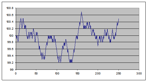
Then plot the result (highlight columns A&B, then "Insert\Chart\XY (Scatter)"); here's one of mine:
|
Matlab First, S0 = 100; % initial price TT = 250; % number of trading days
Then, stockprice = zeros(1,TT); stockprice(1) = S0;
And we model the "up or down by a ten bps" with the "unifrnd(0,1)" command, which selects a random number between zero and one. If it's greater than 0.5 then we assume the price goes up; if less than 0.5 then the price falls.
So this evolution of the price would be: is_up = unifrnd(0,1) > 0.5; % one if up; zero if down is_down = ~is_up; % is zero everywhere is_up is one and vice versa
Of course this isn't very realistic, but it's a start.
So have the computer walk through a year's time like this: for indx = 2:TT % 250 trading days is_up = unifrnd(0,1) > 0.5; % one if up; zero if down is_down = ~is_up; % stockprice(indx) = stockprice(indx-1)*(1 + 0.001*(is_up - is_down)); end
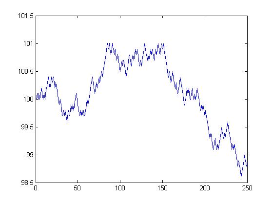
Then see what it looks like: plot(stockprice) This is one of mine:
(this is program mod_stock_l6a.m)
|
|
Simple, right?
That's only one run; we might want to see more to get an idea of all of the possible outcomes.
|
|
|
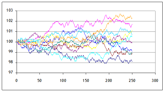
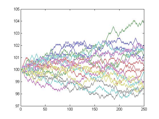
Here are 10 series (copied and pasted the whole S, "up," and "down" 10 times),
|
To do this in Matlab, we first create a big matrix to hold all of the stock price paths: possib_pr = zeros(TT,20); % 20 possible paths And then put another loop around the first one that we wrote (remembering to save the results of the price evolution into the big matrix).
for out_indx = 1:20 stockprice = zeros(1,TT); stockprice(1) = S0; for indx = 2:TT % 250 trading days is_up = unifrnd(0,1) > 0.5; % one if up; zero if down is_down = ~is_up; % is zero everywhere is_up is one and vice versa stockprice(indx) = stockprice(indx-1) * (1 + 0.001*(is_up - is_down)); end possib_pr(:,out_indx) = stockprice'; % puts the 250 days into a column of 'possible price paths' end
Then, again, plot the output. plot(possib_pr)
|
We're not done yet; we can make it better. But the real point for now is to see the basic principle of the thing: we can simulate stock price paths as random trips.
The changes each day are
still too regular each day is 10 bps up or down; never constant,
never bigger or smaller. That's not a
great model for the middle parts. But
the regularity within each individual series does not necessarily mean that the
final prices (at step 250) are all that unrealistic.
I ran 2000 simulations; this is a histogram of the final price of the stock:
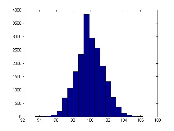
It shouldn't be a surprise
that it looks rather normal (it is the result of a series of Bernoulli trials that's what the Law of Large Numbers says
should happen!).
With computing power being so cheap (those 2000 simulations of 250 steps each took far under a minute even on my slow laptop) these sorts of models are very popular (in their more sophisticated versions).
It might seem more "realistic" if we thought of each of the 250 tics as being a portion of a day. ("Realistic" is a relative term; there's a joke that economists, like artists, tend to fall in love with their models.)
There are times (e.g.
|
Tree Models |
|
|
From
One way of solving problems of option valuation is to split the problem into tiny steps: first, suppose that the stock would either rise or fall by some discrete amount. Of course this is a terrible assumption if we're talking about a period of time like 3 months, but it's not a bad assumption is we're talking about a period of time like a second. And if we can solve it, then we can model the first second, then the next and the next, up to three months! (Or, we might not have that many steps, but at least we can have enough to get a decent approximation.) The full model is called a tree, because each branch splits into more branches and so on.
But first we have to solve the 2-step tree. Suppose the stock is worth 100. Either it goes up to 110 or down to 90 after a time interval. This tree would be drawn like this:
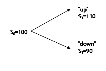
The upper node has a value
of 110 and the lower node has value of 90.
There is some probability of going up or down (in our first simple model
we set this probability to but it could take any value from zero to 1);
it is adequate to specify just one probability in this simple case since pdown
= 1
pup.
There is also a riskless
asset, a bond, that can be purchased at price of 1 today and will payoff (1+R)
after a year this is just a formalization of the idea that
agents can borrow and lend at LIBOR.
Binomial Model
explanation from Tomas Björk book
Two assets, Bt and St
2 times, 0 & 1
B0 = 1, B1 = 1 + R
S0 = s,
,
with probability pu and pd;
alternately
,
where
A portfolio is (x,y), x units of Bond and y units of Stock,
Assume x, y can be any real number; no transactions cost or bid/ask spread
Value of a portfolio is Vt = xBt + ySt
so V0 = x + ys, V1 = x(1+R) + ysZ
Arbitrage portfolio would have V0 = 0 but V1>0
Arbitrage free means d ≤ (1 + R) ≤ u
Implies that (1+R) is a linear combination of d & u;
i.e. there are some α, β such at
(1+R) = αd + βu, α+β=1, α>=0, β>=0
or, alternately,
(1+R) = qd d + qu u, qd + qu = 1, qu>=0, qd>=0, if we interpret as 'probabilities' under EQ
this is "risk-neutral probability" or "martingale" probability
can calculate these risk-neutral probabilities with a bit of algebra,
Then any contingent claim, G(Z), can be priced with the risk-neutral probabilities as
To show this, want to find some portfolio that has the same value as G(Z) at time 1; so
which means finding x and y such that
(1 + R)x + suy = G(u)
(1 + R)x + sdy = G(d)
These solutions are:
So option values are
calculated as if in a risk-neutral
world but of course this is not an actual
description of the world, nor need it be.
Also hold for all investors whether risk-neutral or otherwise.
Example: Stock is worth 100
now; it goes up to 110 (so u=1.1) with probability 70% (pu = 0.7) or
goes down to 90 (d=0.9) with probability 30% (pd = 0.3). A call has strike of 105 so it is worth
either 5 or 0. Assume R=0 to make things
really simple. So from the definition of
qu and qd, we have (1+R) = qd d + qu
u, qd + qu = 1; the first equation becomes 1 = 1.1qu
+ .9qd, so qd=qu=0.5. From this we find that the price, G0,
of the call with value of 5 or 0, is EQ[G1] = qu*5
+ qd*0 = 2.5. This seems odd
since the option has a 70% chance of expiring in the money shouldn't it be worth at least $3.50?! But the $2.50 price comes from the
risk-neutral rate not the actual probabilities.
Why is this? Because the portfolio
(paying off $5 if "u" and $0 if "d") can be replicated by
holding (x,y) units of (bonds, stocks).
How many? Plug into the formula
above or solve: if "u" then x(1+R) + ysu = G(u), or x+110y = 5. If "d" then x(1+R) + ysd = G(d) or
x + 90y = 0, so subtract the second equation from the first and get y= 5/20 =
. Then x = -22.50. A portfolio that is short 22.5 bonds and long
of a stock has initial price of x+ys = -22.5 +
(100)
= 2.50. If the stock goes up then the
portfolio has value -22.5 +
(110)
= 5; if the stock goes down then the portfolio has value -22.5 +
(90)
= 0. So this portfolio replicates the
option payout. If some sucker were to
offer to buy options at $3.50 (thinking that, since he has a 70% chance of
making $5, that seems like a good bet) then I could create as many options as I
want (at a cost of $2.50 each) and sell them for $3.50. (Create the option with the opposite holding
of the replicating portfolio: long 22.5 bond units and short
of a stock would pay out 22.5
(110)
= 5 if "up" and pay out 22.5
(90)
if "down".)
Now do for R=0.02 will the option be more or less expensive?
Alternate Derivation, using
We return to the previous model, with a stock worth 100 currently, which either goes up to 110 or down to 90 after 6 months.
Suppose I have a short
position in a call with strike of 100 (ATM) and I want enough stock to make the
total portfolio riskless between the two nodes.
How much stock does it take? Call
it "". If the stock rises to 110 then I would have
110*
worth of shares minus 10 for the short call, for total 110
- 10. If the stock went down to 90 then
I would have a portfolio worth 90
. What delta would give the same payoff in each
state? Set 110
- 10 = 90
so
=10/20
= 0.5. So a portfolio with a half share
of stock and one short call would always have the same payoff (either 55
10 if the stock goes to the up node or 45 if
the stock goes to the down node) so its value must grow at the risk-free rate
interest rate
or else there would be arbitrage
opportunities, if there were 2 portfolios with the same (riskless) payoff but
different values.
Here we'll slip into
continuous-time interest, so the present value of this payoff in 6 months had
better be 45e-rT = 45e-0.5r. If the current risk-free six-month zero rate
is 4.5% then this is 45e-0.045*0.5 = 45e-0.0225 = 45*
0.97775 = 43.9988. So the current value
of this portfolio .5*S0 c = .5*100
c = 50
c must equal 43.9988 so c = 6.001.
Generalize this to a stock
that moves either up by some amount "u" or down by "d" (so
u > 1 and d < 1). So the value of
a portfolio, with shares of the stock, is either uS0
or dS0
. Also assume that we have a short position in
one option that has value of fu or fd, if the stock goes
up or down. So the portfolio value in
the "up" node is uS0
- fu; the portfolio in the "down" case is dS0
- fd. We can find a value of
that makes the portfolio riskless; i.e. find
such that uS0
- fu = dS0
- fd or
(
from the previous notation).
Denote f as the current
value of the option, so we must have that S0
- f = e-rT(uS0
fu) and f = S0
(1
ue-rT) + e-RTfu. Some more algebra (plus the equation for
) gives us that
.
(Compare with above, in the discrete-compounding example, where we have (1+R) instead of eR but no other real difference in the formulas.)
In a risk-neutral world,
the p and (1 p) terms can be interpreted as the
probabilities of an up or down movement, so that the tree can be sketched as:
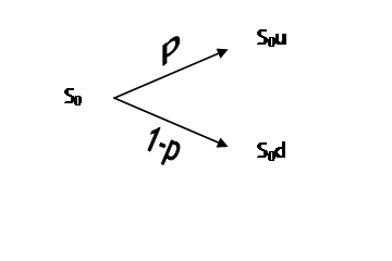 .
.
Although, again these "p" are risk-neutral probabilities NOT real probabilities in the world.
Now suppose that the six months were divided into two steps: U or D and then another u or d again (so we could have any of the sequences Uu, Ud, Du, or Dd). Typically we would allow the tree to be "recombining" so that Ud and Du get us to the same place:
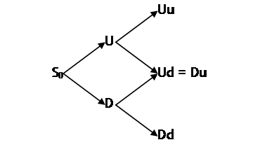 , which is equivalent to setting each up or down movement to
the same factor: U=u at each step and D=d at each step. So a stock that initially went up from S0
would be worth US0; if it then fell it would be US0d. If it went first down then up, it would be DS0u;
if u=U and d=D then these are evidently the exact same numbers!
, which is equivalent to setting each up or down movement to
the same factor: U=u at each step and D=d at each step. So a stock that initially went up from S0
would be worth US0; if it then fell it would be US0d. If it went first down then up, it would be DS0u;
if u=U and d=D then these are evidently the exact same numbers!
We take the time interval
at each step to be ,
where m is the number of steps in the tree.
Then solve the tree backwards (from right to left)
the final nodes are the simple two-step trees
that we just solved; do the whole last column of two-step trees, then back up
and use the answers just found to solve the next-to-last column.
Puts work the same way as calls. Trees are often used to value American options or other more exotic options (that are path-dependent) since at each node the computer can check whether early exercise is optimal.
For trees with more than a very few outcomes, this calculation becomes boring and is best suited for a computer. Back in the old days, a thirty-step tree might have been considered to be pretty awesome; as computing power keeps increasing the number of possible steps can be increased as well (with diminishing returns, of course).
How do we create
"good" tree models? As we go
on, we will discuss the volatility of the stock, σ. Generally we
set and
.
While we're talking about ,
let's mention "delta".
Financial practitioners sometimes talk about "doing the
Greeks" or other such expressions.
Delta,
,
is the first important concept: how many shares of stock must be held, per
option held, to create a riskless hedge.
(Sometimes called delta hedging.)
In general delta will change over time.
A company that wants to keep a hedged portfolio must balance the costs
of rebalancing with the benefits of keeping a close hedge.
Numerical Examples
First show that the
probability case gives the same answers for the call option as does the
risk-free no-arbitrage argument. The
stock has a p chance (in the risk-neutral world) of moving up to 110 and a (1 p) chance of going down to 90 so its expected
value is 110p + 90(1
p) which must be equal to 100erT. (Note
there is no negative sign there!) The p that solves this equation is
-- again, note that this probability is
determined entirely by the risk-free rate and the up/down values, NOT the
actual probability of occurrence. The
call has a payoff of 10 in "up" and zero in down so its expected
payoff (under the risk-neutral probability) is 10p = 6.13. The present value of this is 6.13e-rT
= 6.001. This is precisely the answer
recorded above.
We can work the trees with
other options (puts, American options, various other derivatives). For example, return to the one-step tree,
with S0 = 100, uS0 = 110, and dS0 = 90. What if we had a put option at the
money? It would have a zero payoff in
"up" and a payoff of 10 in "down". So the portfolio that is short the put and
has of the stock would return 110
in "up" and 90
- 10 in "down". Set these
equal and find
= -0.5.
Yes, it's negative: that means the portfolio should be short a half
share of stock. The riskless portfolio
returns -55 at the end of the period so its present value is -55e-rT. The portfolio is currently worth -0.5S0
p = -55e-rT so that p = 55e-rT
- .5S0. With T=0.5 and
r=0.045 (just like the first example) this is 53.776
50 = 3.776.
(Recall the put-call parity
formula, c p = S0
Ke-rT, does that check out? Yes:
6.0012
3.776 = 100
100e-rT = 100
97.775 = 2.225.)
If the put had a different
strike price, say of 97.50, then we would still follow the same procedure. This put would payoff 7.50 in
"down" so the portfolio that is short the put and with of the stock would return 110
or 90
- 7.5 so
= 7.5/20 = - 0.375. This riskless portfolio would have present
value of -41.25e-rT, which we would set equal to the current market
value of -0.375S0
p = -37.5
p.
Solve to find p = 2.832.
Now let's try a 2-step model. Still keep S0 = 100. Now let the percent change be 5% so first the stock either rises to 105 or falls to 95; then it moves to 110.25, 99.75, or 90.25 (as shown in the table below). We won't worry that the center node is no longer precisely 100 since that's not important for this exercise.
|
|
|
110.25 |
|
|
105 |
|
|
100 |
|
99.75 |
|
|
95 |
|
|
|
|
90.25 |
Now T = 0.25 because it takes two steps to get to a half of a year; still keep r = 0.045. Consider a call option with strike price of 100. Its value at each node is now shown below the stock price:
|
|
|
110.25 |
|
|
|
10.25 |
|
|
105 |
|
|
|
? |
|
|
100 |
|
99.75 |
|
? |
|
0 |
|
|
95 |
|
|
|
0 |
|
|
|
|
90.25 |
|
|
|
0 |
Since two of the last three
nodes are zero, the option price, when the stock price is 95, is zero. We only need to calculate the top branch of
the tree. So figure what gives 110.25
- 10.25 = 99.75
,
which gives
= 0.976.
So the portfolio is 105
- c =
99.75e-rT
= (0.976)99.75e-0.045*0.25 = 96.286.
So c = 6.214. Put this into the
tree:
|
|
|
110.25 |
|
|
|
10.25 |
|
|
105 |
|
|
|
6.214 |
|
|
100 |
|
99.75 |
|
? |
|
0 |
|
|
95 |
|
|
|
0 |
|
|
|
|
90.25 |
|
|
|
0 |
Now we need only solve the one-step tree, with stock price and option values:
|
|
105 |
|
|
6.214 |
|
100 |
|
|
? |
|
|
|
95 |
|
|
0 |
Now, with a different
delta, we set 105
- 6.214 = 95
;
= 0.6214.
This riskless portfolio, .6214*100
c, must have value of e-rT(95
)
= 58.376. So c = 3.768. The complete tree is:
|
|
|
110.25 |
|
|
|
10.25 |
|
|
105 |
|
|
|
6.21433 |
|
|
100 |
|
99.75 |
|
3.767599 |
|
0 |
|
|
95 |
|
|
|
0 |
|
|
|
|
90.25 |
|
|
|
0 |
Finally, if you know your
statistics you'll recall that repeated binomial statistical draws converge in
probability to a normal distribution (
|
Tree Examples |
|
|
- Stock is currently 10, goes up to 11 or down to 9 after 1 year, rate is 3%. What is value of call with K=10.50? Put with K=9.50?
So
u=1.1 and d=0.9, exp(1*0.03)= 1.03045. Solve 1.03045 = qdd + quu,
qd + qu = 1 to get 1.03045 = qdd + (1- qd)u,
1.03045 = 0.9qd + 1.1(1 - qd), 1.1 1.03045 = .2q to find qd = 0.3477,
so qu = .6523. Alternately
could solve, as in
Or
delta-hedging method has some amount of stock, ,
such that value of 11
- 0.5 = 9
. So
=0.25
(thus 11
=2.75
and 9
=2.25). So PV of this riskless portfolio must be
exp(-.03)*2.25 = 2.1835. So 10
- c = 2.1835 and c=.3165.
If both had the same strike we could check Put-Call Parity, if c-p = S-Ke-rt (it does check out).
- Stock was at 200/$. It was considered that, in 1 month, it could have gone to 190 or 210. So u= 1.05 and d=.95. If the interest rate (was 4%, what were ATM calls and puts valued?
Again
start with exp(rT), now equal to 1.0033.
Set this equal to qd + (1-q)u so 1.0033 = .95q + 1.05(1-q) and 1.05 1.0033 = .1q so q=.4666 and (1-q) is
.5334. So EQ(call) = 10*.5334
= 5.3339; PV(EQ(call))=5.3161.
EQ(put) = 10*.4666 = 4.6661; PV(EQ(put)) = 4.6506.
Or
by -hedging
so 210
- 10 = 190
;
=.5
so portfolio is worth PV(95) = 94.6839, which is currently equal to 200
- c, so c=5.3161 again.
- Next if zoom went to 180, now considered that in a month could be 170 or 190, and interest rate is 2%, what are ATM calls & puts?
Now exp(rT) = 1.0017. Set this equal to qd + (1-q)u so 1.0017 = .9444q + 1.0556(1-q) and q=.4850, (1-q) = .5150. So ATM call is worth PV(EQ(10)) = exp(-(1/12).02) * .5150 * 10 = 5.1415; ATM put is 4.8418.