|
Lecture Notes 7, Wiener Processes and Itô's Lemma K Foster, CCNY, Spring 2010 |
|
|
Learning Outcomes (not directly from CFA exam for this one)
Students will be able to:
§ see how we use Itô's Lemma and the underlying stochastic calculus to set up the Black-Scholes-Merton option pricing result;
Basic Calculus
Recall from basic calculus the definition of the derivative: examine the limit,
and if both the left-hand-side (lhs) and right-hand-side (rhs) limits are equal, then we call this limit the derivative,
.
Re-write this to show that, for very small values of h,
,
or, in a switch of notation, replacing h with Δx,
.
This we can interpret along
the lines of the Taylor Theorem, that for small values of x,
the term
xf'(x)
is a good approximation to
f.
The Taylor Theorem says that for a differentiable function, we can approximate local changes with derivative(s),
Which relates to the
interpretation of the derivative above as basically stating that (since of
course 1! = 1) the first two terms are a 'pretty good' approximation to the
value of the function at f. We can usually think of the
x2
and
x3
and higher-order terms as going fast towards zero, so fast that they are of
negligible importance.
Recall/Learn from Advanced Calc
If we have a function of two variables, say a production function that output is made by two inputs, capital and labor, then we would write this as
and then define the
marginal productivity of each input separately, as the amount by which output
would increase if one input were increased but the other input held
constant. This is notated mathematically
as . If we had some general polynomial function to
represent output, say that
(a funny-looking production function, I know,
but the math works out easy). Then
and
.
The total differential, dy, is defined as equal to the sum of the partials,
.
This has an easy economic interpretation: if L goes up by a little bit, ΔL, how much does output change? By MPL*ΔL. If K goes up by ΔK, then output rises by MPK*ΔK. If both L and K change by small amounts then we get the total differential above.
Now since we are
suppressing the functional notation, we could write the total differential,
more cumbersomely but equivalently, as . This is useful because, to find the second
derivative, we need to find how the partial derivative with respect to L
changes as K changes (i.e. how the marginal productivity of labor is affected
by having more capital) as well as vice versa (how the marginal productivity of
capital changes with having more labor
i.e. how the partial derivative with respect
to K changes with L. So it is natural to
consider the second partial derivative just like a regular second derivative.
To put this into a bit more
generality, given G(x,y) then .
What if, now, we have a chain of functions, so the function, G( ), is a function of time, t, and another function, X(t)? In finance it is natural to think of G( ) as a payoff function of a derivative that depends on the time (whether it is at expiration) and the stock price (itself a function of time). But for now just allow G(t,X(t)) a general existence. Then we can express the change in the value of the function as
where since X is itself a function of time we can write
,
or, in full functional notation,
,
which makes clearer that we first take the partial with respect to the first argument, then take the partial with respect to the second argument (which is itself a function so we use the Chain Rule).
So we've got some fearsome-looking math notation but we haven't done anything more sophisticated than using the Chain Rule.
Next we review some basic statistics that you learned.
Basic Stats
Recall the definition of the sample variance, that
which estimates the true population variance, which is
And note that if the mean is zero, µ=0, then the variance is equal to the expected value of the squared random variable;
.
In statistics it is often
convenient to use a normal distribution, the bell-shaped distribution that
arises in many circumstances. It is
useful because the (properly scaled) mean of independent random draws of many
other statistical distributions will tend toward a normal distribution this is the Central Limit Theorem.
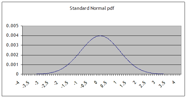
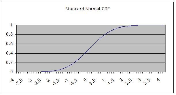
Some basic facts and notation: a normal distribution with mean µ and standard deviation σ is denoted N(µ,σ). (The variance is the square of the standard deviation, σ2.) The Standard Normal distribution is when µ=0 and σ=1; its probability density function (pdf) is denoted pdfN(x); the cumulative density function (CDF) is cdfN(x) or sometimes Nor(x). This is a graph of the pdf (the height at any point):
and this is the CDF:
One of the basic properties of the normal distribution is that, if X is distributed normally with mean µ and standard deviation σ, then Y = A + bX is also distributed normally, with mean (A + µ) and standard deviation bσ. We will use this particularly when we "standardize" a sample: by subtracting its mean and dividing by its standard deviation, the result should be distributed with mean zero and standard deviation 1.
Oppositely, if we are
creating random variables with a standard deviation, we can take random numbers
with a N(0,1) distribution, multiply by the desired standard deviation, and add
the desired mean, to get normal random numbers with any mean or standard
deviation. In Excel, you can create
normally distributed random numbers by using the RAND() function to generate uniform random numbers on [0,1], then NORMSINV(
In Matlab, of course, we
can use x
= random('
Now for the Main Act
I'm going to do some (more)
rather sloppy math here, in the interests of communicating the concept rather
than all of the details. We'll go
through
In simple modeling of stock
prices we had a return in two parts: a general drift and an error. We can represent the return on a security as ,
where the term, aΔt, is the drift and b
W
is an error term. Focus on the error,
W.
For a first approximation we might use the normal distribution to model this error. We want it to have a zero mean or else there would be arbitrage opportunities. Then we want to think of how our uncertainty about a stock value changes with the time horizon; it seems reasonable that as a future date gets farther off, our uncertainty would increase. The range of variation that I expect a stock to be in, after one year, is much larger than the range I'd expect after just a day.
This is equivalent to
assuming that ΔW is normally distributed with mean zero and variance equal to
the distance between time increments, so . The W notation is used since these are called
Wiener processes: it is continuous everywhere but no-where differentiable. It is commonly used in many physical
sciences.
Side Note: The basic property, that the distribution is normal whatever the time interval, is what makes the normal distribution {and related functions, called Lévy distributions} special. Most distributions would not have this property so daily changes could have different distributions than weekly, monthly, quarterly, yearly, or whatever!
We can keep doing this on
and on, finding that the variance at a point half-way there is half of the
original variance like Zeno's famous paradox of Achilles and the
tortoise.
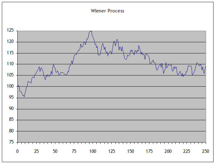
With some mathematical hocus-pocus we can prove that this converges to a Wiener process. This could look something like this:
Recall from calculus the
idea that some functions are not differentiable in places they take a turn that is so sharp that, if we
were to approximate the slope of the function coming at it from right or left,
we would get very different answers. The
function,
,
is an example: at zero the left-hand derivative is -1; the right-hand
derivative is 1. It is not
differentiable at zero
it turns so sharply that it cannot be well
approximated by local values. But it is
continuous
it can be continuous even if it is not
differentiable.
Now suppose I had a
function that was everywhere continuous but nowhere differentiable at every point it turns so sharply as to be
unpredictable given past values. Various
such functions have been derived by mathematicians, who call it a Wiener
process (it generates Brownian motion).
(When Einstein visited CCNY in 1905 he discussed his paper using
Brownian motion to explain the movements of tiny particles in water, that are
randomly bumped around by water molecules.)
This function has many interesting properties
including an important link with the Normal
distribution. The Normal distribution
gives just the right degree of variation to allow continuity
other distributions would not be continuous or
would have infinite variance.
Note also that a Wiener
process has geometric form that is independent of scale or orientation a Wiener process showing each day in the year
cannot be distinguished from a Wiener process showing each minute in another
time frame. As we noted above, price
changes for any time interval are normal, whether the interval is minutely,
daily, yearly, or whatever. These are
fractals, curious beasts described by mathematicians such as Mandelbrot,
because normal variables added together are still normal. (You can read Mandelbrot's 1963 paper in the
Journal of Business, which you can download from JStor
he argues that Wiener processes are
unrealistic for modeling financial returns and proposes further
generalizations.)
These Wiener processes have
some odd properties. Return to the
notion of approximating a smooth process by a ,
we want to find
. Then the
or,
where we can approximate G
as its first derivative, times the size of the step,
x. And the existence of the derivative means
that, in a sense, the second order and higher terms are very small
small enough that the first derivative is the
limit as the size of the step goes to zero.
As we noted, Wiener processes are not differentiable. This is largely because of the second-order term: the random variation is "too big". But we can try to figure out a way to take account of the second-order term.
We argued intuitively that
the variance of the Wiener process is ,
that the variation is proportional to the time step. In our recollection of basic statistics we
said that the variance of any mean-zero random variable is
;
this implies that
. Looking at the equation above, showing the
it is of magnitude
t. Since
this means that the second-order Wiener
process term is of the same order as the first-order drift term.
Being a bit more careful,
we can start from and then just idly find
. Again the variance of
W
is of a higher order,
,
that the variance of the Wiener process is given as the size of the
time-step. So
. The middle tern does, however, drop out since
Δt and ΔW are each very small, and multiplying two very small things (which are
uncorrelated) by each other will give an even smaller result. The ΔW2 term doesn't drop the same
way because ΔW is correlated with itself (its variance).
So returning to the
,
or, switching from
.
Now substitute our basic
definition of ,
as well as our deduction above that
,
so
.
This is a genuinely weird result. Stop a moment and consider it: the variance, b, of the underlying process, suddenly emerges to have a direct influence on the level of G (since it multiplies by Δt).
This is the beginning of the larger result, known as Itô's Lemma.
We might wish to analyze a
more general function, say . This is a good representation of the payoff
to a derivative, since it depends on t (time to expiration) as well as the
value of the underlying security, x(t).
We'll move to a continuous time representation of x and write
(with "d" instead of Δ).
In this case the first
order partial derivatives are . We can omit the second order terms from the
first arguments since these are of order
. But the second order terms from the second
argument is
where, as we previously found,
so the second-order term is
. So the total derivative of G, dG, is
and then we substitute in
the term to get
.
And that ugly bit of
mathematics is Itô's Lemma. It shows a
general formula for how the first order effect (the expected value) is affected
by the second-order terms not just the variance but also the second
"derivative" of the function of the Wiener process.
To take the most ordinary
instance, take ,
so the x are price changes and G(x) gives the value of the stock. Then
and
;
of course
. Substitute these into Itô's Lemma to find
Since this beast that we're
calling is the stock price,
,
we can re-write the equation as
,
which shows that the mean of the stock price return is determined in part by the variance.
One of the other basic properties of Wiener processes is that they have a Markov property (or representation). This means that their history is irrelevant: the current value gives the best forecast. This coincides with our model of weak stock market efficiency, the theory that current prices embody all possible information. If there were useful information to be derived from the stock's history, then someone else would have likely already found it and used it.
Formally, z is a Wiener process if:
- the change, z = (zT-zt), over a short period of time,t=(T-t), is, whereand
- all of the z terms over different time periods are independent.
So if we define N = T/t,
then zT =z0 +
.
A generalized Wiener process adds a drift rate that is a known function and a variance function, so now x is a generalized Wiener process, dependent on z, a standard Wiener process, if dx = a dt + b dz, where a and b are constants..
An Itô process is a further
generalization, where now a and b are given functions of x and t, so ;
for short discrete changes we assume that a and b are constant over some range
so that approximately
,
where you will note that we've inserted the identity that
.
We often model a stock's
percentage return as a generalized Wiener or Itô process, dS = µSdt + σSdz, or dS/S = µdt + σdz; in discrete time this is S/S
= µ
t
+ σε
.
Itô's Lemma
If we have a function,
G(x), where x is an Itô process, ,
then Itô's Lemma just tells us that finding
G(x)
is more complicated:
.
This requires a good bit of calculus to get your arms around. If you recall the math, good. If not, just remember the formula and keep this around so that after you take some more math classes you can come back to Mr. Itô and his Lemma.
Recall from calculus how to
find a Taylor expansion, for some function G(x), which is near G(x0)
so we want to find G
= G(x)
G(x0):
;
that G is differentiable means that the higher-order terms (
x2
and up) are tiny so we have a good approximation.
Next, if G were a function of both x and y, G(x,y), then the total derivative is:
Normally, a function that
is differentiable has the higher-order powers (x2
and
y2
and
x
y)
again die off at a high rate so we would be left with just the terms involving
x
and
y.
Now if this function, G(x),
has an x that is an Itô process, ,
or, if we drop some of the extra notation, that
;
in discrete time this is
.
Itô's Lemma tells us that
finding G(x)
is more complicated, that
. It might be easier to remember if we break it
into the relevant parts: if we did not have a stochastic component, then if we
differentiated G(x(t,z),t) then we'd have
;
then Itô's Lemma just adds in a term,
.
How can we show this?
Normally we could drop the
second-order terms because we're letting the dx and dt terms get
infinitesimally small so that (x)2
and (
t)2
get even tinier. But in this case,
so
. How is the last term different from the first
two? It does not have
t
to any higher power (squared or to the 1.5 power). So it doesn't drop out
we have to incorporate it into the
and substitute it into the
.
From here we just
simplify. If then its variance is one so the expected value
of ε2
=1 and that term drops out. Also we substitute in
and so
,
or, rearranging,
That is the result that you were promised at the beginning of this section. Congratulations if you made it this far!