|
Lecture
Notes 8, Black-Scholes-Merton Option Valuation – 3
separate explanations! K Foster,
CCNY, Spring 2010 |
|
|
Learning Outcomes (from CFA exam)
Students
will be able to:
§ explain the assumptions underlying the Black–Scholes–Merton model and their limitations;
§ use the Black-Scholes-Merton model to
calculate options prices;
From
The Black-Scholes-Merton formula is one of the highlights of finance
theory. Mark Rubinstein, past president
of the American Finance Association, described it as, "one of the most
successful in the social sciences and has perhaps … the most widely used
formula, with embedded probabilities, in human history" (Journal of Finance, 49(3), p. 772). Nonetheless, it can be frustrating to learn
it, since the key formula seems pulled out of thin air to solve a differential
equation. You can read the original
articles (from JStor in the library):
Black, Fischer, and Myron Scholes, (1973).
"The Pricing of Options and Corporate Liabilities," The Journal of Political Economy, 81(3),
637-54.
Merton, Robert C., (1973). "Theory of Rational Option
Pricing," The
Assume that VS is Wiener process, VS = µSdt + sSdz
If this is a
model of a stock price then we want to look at how the returns vary, where the
percentage return is (S1 - S0)/S0 = ∆S/S
and from calculus, the derivative of ln(S) is dS/S or ∆S/S.
So first
find the distribution of ln(S). By Itô's Lemma:
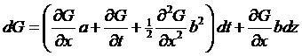
we have to
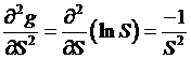
find the first and second derivatives of ln(S):
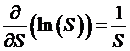 ,
, 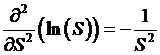 , and of course
 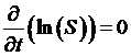 , so that:
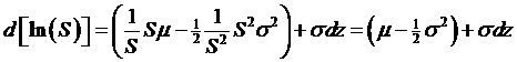 .
.
This
probably doesn't seem intuitive at all: why do we need to subtract off a term
for the volatility?
Nonetheless,
this implies that ln(S) has a normal distribution,
which can also be stated as S has a log-normal distribution. If a normal distribution looks like this:
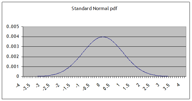
a log-normal
distribution looks like this:
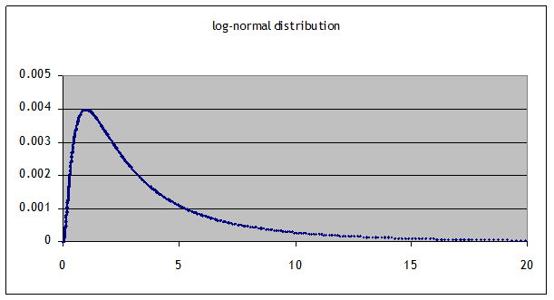
since exp(0)
= 1, the median is still at 1 however the mean is skewed to the right. This might seem like a better model for stock
changes: a stock price can never be negative (this defines the limited
liability corporation) but the upside gains can be huge (although with a very
tiny probability).
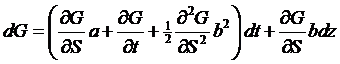
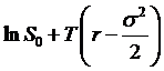
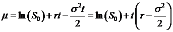
So Itô's Lemma tells us that the distribution of ln(ST) is going to be normal with mean 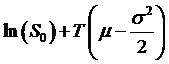 and standard deviation
![]() . Alternately we could
express this by noting that ln(ST) – ln(S0) = ln(ST/S0)
has mean
. Alternately we could
express this by noting that ln(ST) – ln(S0) = ln(ST/S0)
has mean  and the same standard
deviation.
and the same standard
deviation.
Now we want
to figure the distribution of x, where x is the return on a stock over a period
of time,
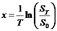 . This is just
dividing through by a constant (T) so the new mean is going to be
. This is just
dividing through by a constant (T) so the new mean is going to be  and the standard
deviation will be
and the standard
deviation will be ![]() .
.
Assumptions of Black-Scholes-Merton model:
- Stock has log-normal
distribution
- Short-selling is permitted
without restrictions
- No transactions costs or taxes
- No riskless arbitrage
opportunities
- Continuous trading of securities
- Riskfree interest rate, r, is constant
for all maturities
Some of
these assumptions will be later relaxed but we'll keep them for now.
Black-Scholes
formulas:
Modify the
intrinsic value formulas (and recall the lower bound formulas) to get something
that looks like the expected present value analogs:
call payoff:
![]()
Remember we
found that it has a lower bound of S0 – Ke-rT,
which in some sense is the present-value analog of its intrinsic value.
From
what we learned about risk-neutral valuation, we might think of taking some
sort of risk-neutral expectation of the call value to find its price; this
might mean finding some probabilities, π1 and π2,
such that
π1S0
- π2Ke-rt
gives the price of
the call. This is an excellent
guess! Figuring out the exact functions
for these probabilities is a bit tricky, but that's what BSM got a Nobel prize
for. The formula just fills in Normal
calls for those probabilities.
call price: ![]()
Similarly for puts,
put payoff: ![]()
has lower bound of Ke-rT - S0 so the BSM formula fills
in probabilities, π3 and π4, in the formula,
π3Ke-rt - π4S0 to get
![]() put price:
put price: ![]() ,
,
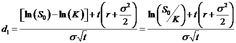
The d1
and d2 parameters can be seen as measuring the location of the
strike price relative to the expected value of the stock. They are the standardized measure of how many
standard deviations from the mean is the value,  . These probabilities
discount the intrinsic value terms for the call and put.
. These probabilities
discount the intrinsic value terms for the call and put.
We are given
a present stock price and a strike price, and we want to figure out how far
away the strike price is, from the likely future value of the stock. How far is far? A few pennies might not be much if the stock
trades at $75 per share but for "penny stocks" it could be a very
long way. It is the volatility that
gives the answer. So we want to take the
distance between S0 and K (actually the natural log of the distance,
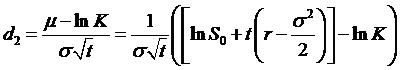
since we're assuming a distribution of returns), {lnS0 – lnK}, subtract the mean (this is the  term), and divide by
the standard deviation.
term), and divide by
the standard deviation.
Consider the
problem graphically from the standpoint of risk-neutral valuation. We have S0 and K, where we assume
that ST is distributed log-normal.
So if we were valuing an out-of-the-money call, we might have something
like this:
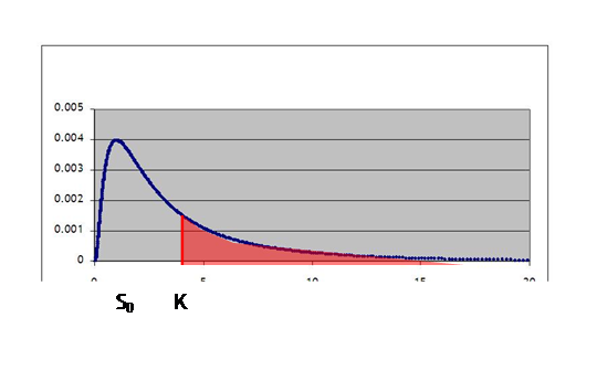
Where the
red shaded area is where the call would pay off. The first step is to translate this
log-normal distribution into a standard normal, which is done by transforming
the mean and variance, so that we get something like:
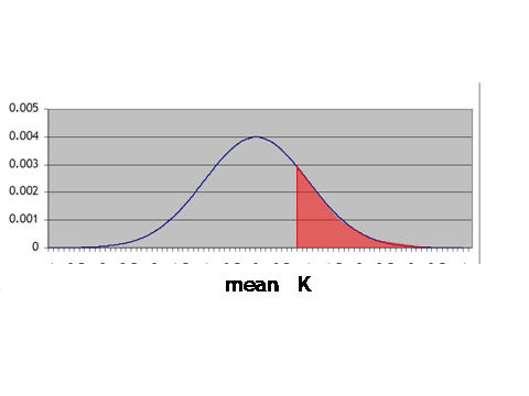
Then we want
to find the expected value of a payoff that starts at zero at K and rises above
that level.
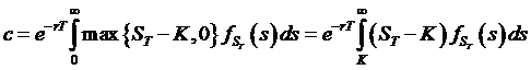
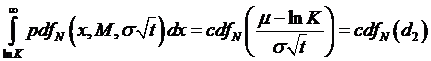
This call
option has value max(ST – K, 0) so its present discounted expected
value is e-rTE[max(ST
– K, 0)], which is ![]() . The reason for the
separate terms d1 and d2 is that they relate to different
expected values: a call option entitles the bearer to get ST if ST>K
but costs K (but no more) if ST>K. If we rewrite the Black-Scholes
formula,
. The reason for the
separate terms d1 and d2 is that they relate to different
expected values: a call option entitles the bearer to get ST if ST>K
but costs K (but no more) if ST>K. If we rewrite the Black-Scholes
formula, ![]() , then the second term is the probability that the stock will
get as high as the strike price, K. The
first term is the probability that the call will return the stock price (i.e.
that it will be above the strike) – and will be zero if not.
, then the second term is the probability that the stock will
get as high as the strike price, K. The
first term is the probability that the call will return the stock price (i.e.
that it will be above the strike) – and will be zero if not.
The Black-Scholes formula is a solution to the Black-Scholes differential equation (which is a form of the heat
equation). Return to the "delta
hedging" argument. We could buy V shares of stock to form a perfect
hedge against the movements of an option.
(Actually it is only a perfect hedge for infinitesimal changes, but for
now we'll elide that problem.) What is
delta? If we label the option price as p
(some price) we of course note that p is a function of the stock value and
time, so we can write p(S,t). So if the stock price changes by VS then the option price will change
by  , so if
  then we have a perfect
hedge. So the position is (VS – p) , or, dividing through by V, (S – p/V).
Since this is a riskless portfolio, it should return rVt (or else there are arbitrage
opportunities). As there are tiny
changes, the value is (dS – dp/V), but we need some stochastic
calculus (Itô's Lemma) to get a value of dp. Recall that
then we have a perfect
hedge. So the position is (VS – p) , or, dividing through by V, (S – p/V).
Since this is a riskless portfolio, it should return rVt (or else there are arbitrage
opportunities). As there are tiny
changes, the value is (dS – dp/V), but we need some stochastic
calculus (Itô's Lemma) to get a value of dp. Recall that
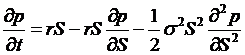
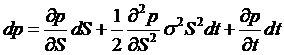 so, substituting back,
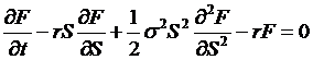
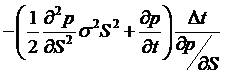 . Set this equal to
the riskfree rate and get
. Set this equal to
the riskfree rate and get
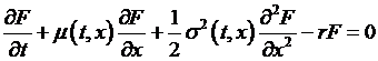
 . There is one
boundary condition, which is the definition of the option, that p(x,T) = payoff (at date T, the expiration date). The solution to this partial differential
equation is the Black-Scholes equation.
. There is one
boundary condition, which is the definition of the option, that p(x,T) = payoff (at date T, the expiration date). The solution to this partial differential
equation is the Black-Scholes equation.
A bit more intuition:
We can check
if the formula results change as we would intuitively expect, given the
different input arguments.
call price: ![]()
put price: ![]() ,
,
where 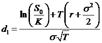 and
and 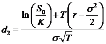 or
or ![]() .
.
The stock
return does not explicitly appear in the formula, except insofar as it affects
the current price. The time-to-maturity
for the option appears only multiplied by the risk-free interest rate and the
volatility, so these aspects are intuitive enough. As time-to-maturity, volatility, or the
risk-free rate increase (T, s, or r), the value of the option rises towards its
intrinsic value.
As
volatility falls toward zero, then if the option is already in the money then
the probability that it will stay there goes towards 1 and the option is worth
the intrinsic value. If the option were
out of the money, then a low volatility means it is less and less likely to
ever be worth more than zero.
As the stock
price rises (S0), it becomes almost certain that the option will be
exercised and the call price rises toward S0 – e-rTK, as
d1 and d2 rise so that cdfN( ) of each of
those gets closer and closer to 1. A put
price would go in the other direction as the stock price rose; again -d1
and -d2 would drive the cdfN( )
terms toward zero.
See the
Excel sheet showing how changes in the parameters affect call and put
prices. (These are "the
Greeks" – but we'll get to that later.)
Implied Volatilities
In practice,
some of the crucial Black-Scholes assumptions are not
true so the formulas are not exact.
However they are nonetheless often used in reverse to generate a
volatility from a given option price. If
an at-the-money call price is $6.46, is that a good or a bad price? It depends on the current price of the stock,
in a nonlinear way. A different way to
price an option is to quote its implied volatility – i.e. that volatility
which, put into the Black-Scholes equation, would
give the price that is "really" being quoted. This may allow a market participant to better
judge whether the price is good or bad by instead asking, is the volatility
reasonable? If the implied volatility is
too high then the price is high; if the implied volatility is low then the
price is low. Note that this is done,
even though everyone knows that the Black-Scholes
model is not the "true" description of option prices! It still provides a handy way of translating
prices.
Of course,
figuring out these volatilities is no small task, since there is no simple
formula. It takes a computer search
program to do it – to guess numbers and then work to improve the guess until it
is within some criterion range.
Relation to Binomial Trees
Finally note
that we would get the same answer by taking a binomial tree model over a fixed
time period but taking more and more ever-smaller steps.
|
Another take on Black-Scholes-Merton |
|
|
The basic
Black-Scholes formula is pretty simple, once we get
used to it. The expected payoff to a
call (for example) at time T is max{ST – K,0}. If the call is not exercised its value is
zero so it only has value if exercised, so the future payoff is STcdfN(d1) - KcdfN (d2), where d1 and d2
indicate the probabilities that the option will be exercised. We know that a risk-neutral no-arbitrage
valuation implies that ST = S0ert so we
replace that to get S0ertcdfN (d1)
- KcdfN (d2), which is the
future value. The present value
multiplies by e-rt to get S0cdfN
(d1) - Ke-rt cdfN (d2).
Remember our
basic argument: given some stock return that follows a Wiener process, dS = µSdt + sSdz, we want to find the distribution of
the function, g(S) = ln(S). Itô's Lemma tells
us that
 ,
,
so we figure
that 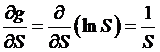 ,
,  ,
,  , a = µS, and b = sS, that
 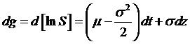 . Since d[lnS] is a Wiener process, we can assert that lnST has a Normal distribution with mean, under
a risk-neutral measure, of
. Since d[lnS] is a Wiener process, we can assert that lnST has a Normal distribution with mean, under
a risk-neutral measure, of
Where did
that ![]() come from? That's the mystery of stochastic calculus.
But there is another way.
come from? That's the mystery of stochastic calculus.
But there is another way.
Jay
Jorgenson and Adriana Espinosa (here at CCNY) have figured out another way to
derive the Black-Scholes-Merton formula, without Itô's Lemma, just some algebra. This summarizes their paper, Espinosa and
Jorgenson (2003).
We assume
that a stock's return is given by:
![]()
Next define ![]() and thus
and thus
![]() ,
,
![]() ,
,
![]()
So that ![]() , which allows us to interpret the
, which allows us to interpret the 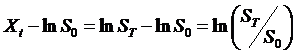 as the percent return;
also note that
as the percent return;
also note that ![]() .
.
We assume
that the ΔS are independent and identically distributed. Independent means that the ΔS at time t
does not depend on the previous day's (or week's or month's) ΔS; the
assumption of identical distribution allows us to assert that its variance is
constant over time. The independence is
a consequence of weak market efficiency, since if the change in stock price
could have been predicted then why wasn't it arbitraged away?
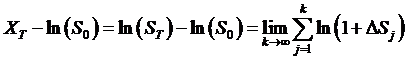
Remember,
from stats, the basic relation that if A and B are independent then the var(A+B) = var(A) + var(B). Now from the
definition of Xt as a sum of independent
but identically distributed terms, we can see that, for any number of little
steps up to time t, the variance of Xt is
![]() ,
,
where, since
theΔS are identical, the variance of ΔS1
is the same as ΔST or any other ΔS – and we'll define this
variance as some constant, s2.
Why all of
this work? Because we might remember the
Central Limit Theorem (CLT) from statistics.
This states that a sum of independent and identically distributed terms
can converge to a distribution, as the number of steps goes higher and
higher. (I use the term "can"
not "must" to remind us that there are a few technical details to be
taken care of, before this is an actual proof, but for now we'll ignore
those.) The Central Limit Theorem allows
us to assert that the distribution goes towards a Normal distribution. The Central Limit Theorem implies:
converges to
a normal distribution with some mean and standard deviation. We have seen that the variance of lnSt must be s2t so that the standard deviation is ![]() , but what is the mean?
, but what is the mean?
To figure
out the mean of this variable, we take a detour through risk-neutral no-arbitrage
pricing. Remember that this argument
contends that
S0 = e-rt E[St],
where the E[
] expected value function uses the probability density function f( ) and is
defined as
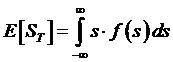 .
.
This doesn't
seem to help since we don't know the distribution function of S so we don't
know the probability density function, f( ).
But the Central Limit Theorem tells us that XT = lnST has a normal distribution, so we would like
to use X instead of S and then integrate with respect to the normal probability
density function rather than some unknown pdf. So we switch the variables X and S by
inserting eX for S (since, by definition, ![]() ), and put in a normal probability distribution,
), and put in a normal probability distribution, ![]() instead of
instead of ![]() to write
to write
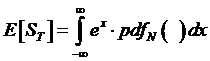 .
.
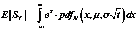
But the
normal probability density function depends on the mean, µ, and standard
deviation, s, so we can write the normal
distribution function as ![]() . We figured out that
the standard deviation is
. We figured out that
the standard deviation is ![]() but what about µ? For now we'll leave it as a variable, and
write:
but what about µ? For now we'll leave it as a variable, and
write:
 , where the function,
 ![]() , is defined as
, is defined as
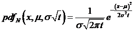 so that
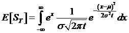
We have an
awful lot of terms with e to some
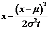
power – can we fix that? Let's
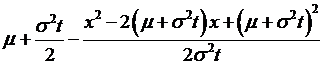
concentrate on the integrand; we see that we are integrating
![]() . We can transform the
exponent as follows:
. We can transform the
exponent as follows:
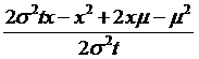
 =
=
= 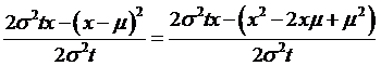
= 
Now what if
we did the ancient mathematician's trick of adding and subtracting a number –
which doesn't change the equality but can transform the variables? So add-and-subtract these terms, 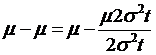
and another  , to get
= 
= 
= 
= 
= 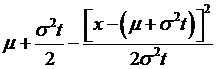
So that we
can re-write 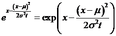 as
as
Why the heck
is that any better? Recall that the
formula for a normal distribution involves  , where M is the mean and S is the standard deviation. The last part of the exp( ) function above
looks like a normal, if we had
, where M is the mean and S is the standard deviation. The last part of the exp( ) function above
looks like a normal, if we had ![]() and
and ![]() .
.
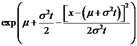
So going
back up to the equation, which had the risk-neutral no-arbitrage value of 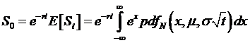 , we replace the integrand with the value found after all of
the algebra to get:
, we replace the integrand with the value found after all of
the algebra to get:
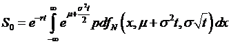
This allows
us to take the ex term that we were integrating out from under the
integral, where it was a pain to deal with.
Now that it's e to the power
of some constant ( ), we can take it to the outside of the integral. Once that's outside the integral, then all
that's left inside is the pdf of a probability
function, and we know that
), we can take it to the outside of the integral. Once that's outside the integral, then all
that's left inside is the pdf of a probability
function, and we know that  so that we get
That's a lot
easier, isn't it?! Then we can take logs
and solve to find that
This is what
Ito's Lemma gave (way back in the beginning), but without the stochastic
calculus. Granted, there's a lot of
algebra instead, but that's more tedious than mystery.
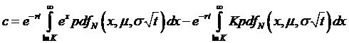
So to price
an option, we just use the expected value formula from above, with the proper
distribution function. A risk-neutral
no-arbitrage argument tells us that a call price, c, must be:
 .
.
Note that
we've eliminated the "max( )" function by just changing the bounds of
integration – this is the conditional expectation now, the expectation of (ST
– K), conditional on if the stock is greater than K.
If we make a
change of variables so that X = ln(S) (thus, S=ex),
then we can switch the probability function from involving ST to
involving ex, which has a distribution that we understand – that's
got mean µ (remember that 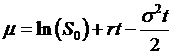 and standard deviation
 ![]() . As part of this
change of variables, we also must change the boundary of integration, now to ln(K). So we get:
. As part of this
change of variables, we also must change the boundary of integration, now to ln(K). So we get:
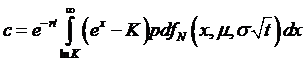 .
.
So now we
break up the pieces and get an integral of ex (which is a problem
that we solved before – we've just got to fix the bound of integration) and an
integral of K, which is a constant and so easy.
So
 , which is
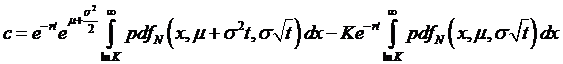 ,
,
and where
the equation with all of the algebra allows us to rewrite the first term to get
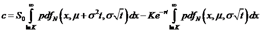
(note that
now the first and second pdf's are different – one
has a transformed mean from the ex simplification and the other does
not). But both pdf's
are pretty simple: they're just integrating over a part of the curve, which is
finding the cumulative distribution, cdfN(
), for some values. So by definition
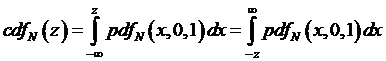 .
.
For a
variable, y, that doesn't have a standard normal distribution (mean zero and
standard error of one), we define 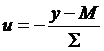 , where M is the mean and
 ![]() is the standard error,
to change variables so that
is the standard error,
to change variables so that
 .
.
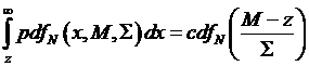
So going
back to the equation for the call price, we evaluate the piece,
 ,
,
where the
term d1 (chosen for no special significance, just by coincidence it
might seem like it could be like the Black-Scholes
formula term d1!) is 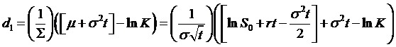
(the last
substitution for µ is from the earlier equation ). This simplifies to
 -- which should look
familiar.
-- which should look
familiar.
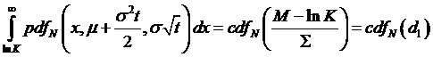
Again going
back to the equation for the call price, we next evaluate the piece,
 ,
,
where now d2
just happens to be
 ,
,
which again
looks familiar.
So the call
price, c is given as
![]() ,
,
which ought
to look real familiar – it's the Black-Scholes-Merton
formula!
|
Yet another take on Black-Scholes-Merton |
|
|
from Björk
This basic
method of finding the BSM model remains fundamentally similar to how we solved
the tree models: show that there is some combination of stock and derivative
that makes a riskless portfolio, so then this portfolio must return the risk-free
rate, so we can value the initial derivative position.
As usual in
solving differential equations, this means pushing around our equation until we
get it into a form that has already been solved by smart people; in this case
this is the Feynman-Kac equation.
Again assume
that there is free and costless trading of any position in the derivative,
stock, and riskless bond.
The
derivative price process changes over time; we label this ![]() since it depends
directly on time and the stock value. As
usual St is the stock price, Bt is the bond price that returns a riskless rate
of return, r, the derivative matures at T, and we model the stock process as
since it depends
directly on time and the stock value. As
usual St is the stock price, Bt is the bond price that returns a riskless rate
of return, r, the derivative matures at T, and we model the stock process as
![]() ,
,
where dW is the driving Wiener process.
Taking the derivative
price as ![]() , we use Itô's Lemma to find the
total differential,
, we use Itô's Lemma to find the
total differential,
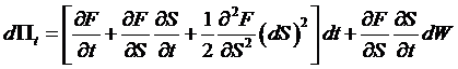 .
.
Then
substitute that  ,
, ![]() , and
, and  , so
, so
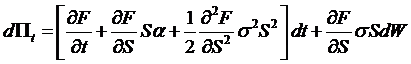 .
.
Rewrite this
into
![]() ,
,
where 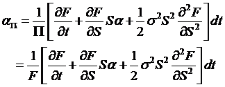 and
and 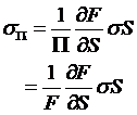 .
.
So now we
have
the bond price process, 
the stock price process, 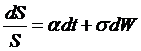 ,
,
and the derivative price
process, 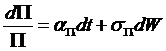 .
.
Next we want
to find some combination of stock and derivative positions that will make a
riskless self-financing portfolio, V.
This means dividing the fraction of the portfolio invested in the stock,
u, and of the fraction invested in the derivative, (1 – u), such that ![]() .
.
Recall that,
from our most basic classes, we understand how to find the growth rate for some
composite based on the growth rates of the parts: if my portfolio is invested ¼
in small-cap stocks and ¾ in large-cap stocks, then the growth of my portfolio
is ¼(growth of small-cap) + ¾(growth of large-cap).
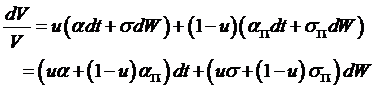
So we can
write 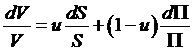 and substitute from
above to write:
and substitute from
above to write:
Now this
portfolio will be riskless if we choose the share invested into stock, u,
correctly so as to zero out the dW term; so choose u
such that ![]() , or
, or  . This is defined as
long as
. This is defined as
long as ![]() , which would only happen if
, which would only happen if  , if the price of the derivative were unrelated to the stock
price – which would be very odd indeed!
So this makes
, if the price of the derivative were unrelated to the stock
price – which would be very odd indeed!
So this makes
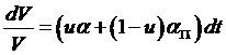 .
.
So if the
value of the portfolio has no random element, then it must grow at the riskless
rate, so  and
and ![]() .
.
Now
substitute in terms, , 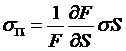 , and
, and 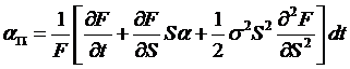 , and note especially that the
  terms drop out – the
derivative price has no dependence on the stock's rate of growth. So we get the equation,
terms drop out – the
derivative price has no dependence on the stock's rate of growth. So we get the equation,
 with the boundary
constraint that, at the expiration date T,
with the boundary
constraint that, at the expiration date T, ![]() .
.
Now for the
casual person reading along, this doesn't look like it's much help, but it
actually is helpful. This is because, as
I mentioned above, somebody else has already a solved tough equation just like
it – it's called Feynman-Kac.
|
Sidebar: The
Feynman-Kac solution sets up the problem from a
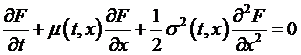
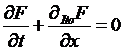
differential equation like this: The
equation might look like a hopeless mess unless we were to remember our Itô calculus and decide that the second part looks like a
part of the derivative when we have to include second-order terms, so we
could write the differential equation as Then
the Feynman-Kac result shows that the solution for
the function, F, that solves this problem is: where
X satisfies It
is a straightforward extension to show that if we had some These
actually allow a much more generalized Itô process
than in the original Black-Scholes-Merton, since
these allow the mean process |
To return to
the original Black-Scholes-Merton problem, we have
the equation
with the boundary
constraint that, at the expiration date T, ![]() . Hooray! This is exactly the formula that the Feynmac-Kac result solves for us, so we don't have to do
extra hard work, they've already done it for us! (Positive externalities of knowledge
capital.)
. Hooray! This is exactly the formula that the Feynmac-Kac result solves for us, so we don't have to do
extra hard work, they've already done it for us! (Positive externalities of knowledge
capital.)
In the
simple case where the mean and variation processes are constants, then we can
write the solution from 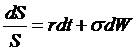 to get the Black-Scholes-Merton formula, that for a call,
![]() ,
,
where 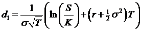 and
and ![]() and
and ![]() is the standard normal
cumulative distribution function.
is the standard normal
cumulative distribution function.