|
Lecture Notes 5 Econ 29000, Principles of Statistics Kevin R Foster, CCNY Spring 2011 |
|
|
Learning Outcomes (from CFA exam Study Session 3, Quantitative Methods)
Students will be able to:
§ define the standard normal distribution, explain how to standardize a random variable, and calculate and interpret probabilities using the standard normal distribution;
The sample average has a normal distribution. This is hugely important for two reasons: one, it allows us to estimate a parameter, and two, because it allows us to start to get a handle on the world and how we might be fooled.
Estimating a parameter
The basic idea is that if we take the average of some sample of data, this average should be a good estimate of the true mean. For many beginning students this idea is so basic and obvious that you never think about when it is a reasonable assumption and when it might not be. For example, one of the causes of the Financial Crisis was that many of the 'quants' (the quantitative modelers) used overly-optimistic models that didn't seriously take account of the fact that financial prices can change dramatically. Most financial returns are not normally distributed! But we'll get more into that later; for now just remember this assumption. Later we'll talk about things like bias and consistency.
Variation around central mean
Knowing that the sample average has a normal distribution also helps us specify the variation involved in the estimation. We often want to look at the difference between two sample averages, since this allows us to tell if there is a useful categorization to be made: are there really two separate groups? Or do they just happen to look different?
How can we try to guard against seeing relationships where, in fact, none actually exist?
To answer this question we must think like statisticians. To "think like a statistician" is to do mental handstands; it often seems like looking at the world upside-down. But as you get used to it, you'll discover how valuable it is. (There is another related question: "What if there really is a relationship but we don't find evidence in the sample?" We'll get to that.)
The first step in "thinking like a statistician" is to ask, What if there were actually no
relationship; zero difference? What would we see?
Consider two random variables, X and Y; we want to see if there is a difference in mean between them. We know that the sample averages are distributed normally so both and are distributed normally. We know additionally that linear functions of normal distributions are normal as well, so is distributed normally. If there were no difference in the means of the two variables then would have a true mean of zero; . But we are not likely to ever see a sample mean of exactly zero! Sometimes we will probably see a positive number, sometimes a negative. How big of a difference would convince us? A big difference would be evidence in favor of different means; a small difference would be evidence against. But, in the phrase of Dierdre McCloskey, "How big is big?"
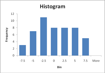
Let's do an example. X and Y are both distributed normally but with a moderately error relative to their mean (a modest signal-to-noise ratio), so X~N(10,3) and Y~N(12,3), with 50 observations.
In our sample the difference is 0.95; =-0.95.
A histogram of these differences shows:
Now we consider a rather strange thing: suppose that there were actually zero difference – what might we see? On the Excel sheet "normal_differences" (nothin' fancy) we look at 1000 repetitions of a sample of 50 observations of X and Y.
A histogram of 1000 possible samples in the case where there was no difference shows this:
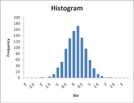
So a difference of -0.95 is smaller than all but 62 of the 1000 random tries. We can say that, if there were actually no difference between X and Y, we would get something from the range of values above. Since we actually estimated -0.95, which is smaller than 62 of 1000, we could say that "there is just a 6.2% chance that X and Y could really have no difference but we'd see such a small value."
Law of Large Numbers
Probability and Statistics have many complications with twists and turns, but it all comes down to just a couple of simple ideas. These simple ideas are not necessarily intuitive – they're not the sort of things that might, at first, seem obvious. But as you get used to them, they'll become your friend.
With computers we can take much of the complicated formulas and derivations and just do simple experiments. Of course an experiment cannot replace a formal proof, but for the purposes of this course you don't need to worry about a formal proof.
One basic idea of statistics is the "Law of Large Numbers" (LLN). The LLN tells us that certain statistics (like the average) will very quickly get very close to the true value, as the size of the random sample increases. This means that if I want to know, say, the fraction of people who are right-handed or left-handed, or the fraction of people who will vote for Politician X versus Y, I don't need to talk with every person in the population.
This is strenuously counter-intuitive. You often hear people complain, "How can the pollsters claim to know so much about voting? They never talked to me!" But they don't have to talk to everyone; they don't even have to talk with very many people. The average of a random sample will "converge" to the true value in the population, as long as a few simple assumptions are satisfied.
Instead of a proof, how about an example? Open an Excel spreadsheet (or OpenOffice Calc, if you're an open-source kid). We are going to simulate the number of people who prefer politician X to Y.
We can do this because Excel has a simple function,
Assume that there are 1000 people in the population, so copy and paste the contents of cells A1 and B1 down to all of the cells A2 through A1000 and B2 through B1000. Now this gives us 1000 people, who are randomly assigned to prefer either politician X or Y. In B1001 you can enter the formula "=SUM(B1:B1000)" which will find out how many people (of 1000) who would vote for Politician X. Go back to cell C1 and enter the formula "=B1001/1000" – this tells you the fraction of people who are actually backing X (not quite equal to the percentage that you set at the beginning, but close).
Next suppose that we did a survey and randomly selected just 30 people for our poll. We know that we won't get the exact right answer, but we want to know "How inaccurate is our answer likely to be?" We can figure that out; again with some formulas or with some computing power.
For my example (shown in the spreadsheet, samples_for_polls.xls) I first randomly
select one of the people in the population with the formula, in cell A3, =ROUND(1+RAND()*999,0). This takes a random number between 0 and 1 (
Next in B3 I write the formula, =INDIRECT(CONCATENATE("population!B",A3)). The inner part, CONCATENATE("population!B",A3), takes the random number that we generated in column A and makes it into a cell reference. So if the random number is 524 then this makes a cell address, population!B524. Then the =INDIRECT(population!B524) tells Excel to operate on it as if it were a cell address and return the value in B524 or the worksheet that I labeled "population".
On the worksheet I then copied these formulas down from A2 to B32 to get a poll of the views of 30 randomly-selected people. Then cell B1 gets the formula, =SUM(B3:B32)/30. This tells me what fraction of the poll support the candidate, if the true population has 45% support. I copied these columns five times to create 5 separate polls. When I ran it (the answers will be different for you), I got 4 polls showing less than 50% support (in a vote, that's the relevant margin) and 1 showing more than 50% support, with a rather wide range of values from 26% to 50%. (If you hit "F9" you will get a re-calculation, which takes a new bunch of random numbers.)
Clearly just 30 people is not a great poll; a larger poll would be more accurate. (Larger polls are also more expensive so polling organizations need to strategize to figure out where the marginal cost of another person in the poll equals the marginal benefit.)
In the problem set, you will be asked to do some similar calculations. If you have some basic computer programming background then you can use a more sophisticated program to do it (to create histograms and other visuals, perhaps). Excel is a donkey – it does the task but slowly and inelegantly.
So we can formulate many different sorts of questions once we have this figured out.
First the question of polls: if we poll 500 people to figure out if they approve or disapprove of the President, what will be the standard error?
With some math (![]() ) we can
figure out a formula for the standard error of the sample average. It is just the standard deviation of the
sample divided by the square root of the sample size. So the sample average is distributed normally
with mean of µ and standard error of . This is sometimes written compactly as .
) we can
figure out a formula for the standard error of the sample average. It is just the standard deviation of the
sample divided by the square root of the sample size. So the sample average is distributed normally
with mean of µ and standard error of . This is sometimes written compactly as .
Sometimes this causes confusion because in calculating the standard error, s, we divided by the square root of (N-1), since , so it seems you're dividing twice. But this is correct: the first division gets us an estimate of the sample's standard deviation; the second division by the square root of N gets us the estimate of the sample average's standard error.
The standardized test statistic (sometimes called Z-score since Z will have a standard normal distribution) is the mean divided by its standard error, . This shows clearly that a larger sample size (bigger N) amplifies differences of from zero (the usual null hypothesis). A small difference, with only a few observations, could be just chance; a small difference, sustained over many observations, is less likely to be just chance.
One of the first things to note about this formula is that, as N rises (as the sample gets larger) the standard error gets smaller – the estimator gets more precise. So if N could rise towards infinity then the sample average would converge to the true mean; we write this as where the means "converges in probability as N goes toward infinity".
So the sample average is unbiased. This simply means that it gets closer and closer to the true value as we get more observations. Generally "unbiased" is a good thing, although later we'll discuss tradeoffs between bias and variance.
Return to the binomial distribution, and its normal approximation. We know that std error has its maximum when p= ½, so if we put in p=0.5 then the standard error of a poll is, at worst, , so more observations give a better approximation. See Excel sheet poll_examples. We'll return to this once we learn a bit more about the standard error of means.
![]() A bit of Math:
A bit of Math:
We want to use our basic knowledge of linear combinations of normally-distributed variables to show that, if a random variable, X, comes from a normal distribution then its average will have a normal distribution with the same mean and the standard deviation of the sample divided by the square root of the sample size,
.
The formula for the average is . Consider first a case where there are just 2 observations. This case looks very similar to our rule about, if , then . With N=2, this is , which has mean , and since each X observation comes from the same distribution then so the mean is (it's unbiased). You can work it out when there are observations.
Now the standard error of the mean is . The covariance is zero because we assume that we're making a random sample. Again since they come from the same distribution, , the standard error is .
With n observations, the mean works out the same and the standard error of the average is .