Lecture Notes 8 Econ 29000, Principles of Statistics Kevin R Foster, CCNY Spring 2011

 

About Midterm:

Midterm is on Friday March 18, 12:30-1:45pm, in either of 2 locations – the NAC Economics computer lab in 6150 and the main NAC computer lab on the ground floor (just the PCs not the Macs).  There are ~30 machines upstairs and ~50 downstairs.  Arrive early to get your pick!  Or bring your own.

 

Exam is open book, open notes, open internet.  The only restriction is on communications, where an answer to the specific problem posed on the exam is requested.  No real-time communication of any type is allowed during the exam.

 

Exam answers can be put on computer or in blue books or any combination.

 

Exams are graded 'blind' so you only identify by your ID number.

 

Extra office hours 4:15-5:15 on Tuesday.

 

More examples: beating Z-stats down to the ground with confidence intervals and p-values.

 

We can straightforwardly change units to go from measuring differences in Z-statistics to using confidence intervals.  Go back to the previous example, with the ATUS data in broad classifications, where we looked at differences in how much time people with different educational qualifications spent with kids.  SPSS gave us this output:

 

Case Summaries
time with children (own and others)
education categories	N	Mean	Std. Deviation
less than high school	4700	47.6104	94.33761
high school diploma	13223	48.9654	89.57632
some college	15465	53.9291	93.87316
college degree	12388	65.2511	101.45307
advanced degree	5796	70.0430	103.82020
Total	51572	56.6112	96.21166

 

We found the difference in time spent with kids, between 20-50 year-olds without a high school diploma and those with a high school diploma, as 47.6104 – 48.9654 = – 1.355.  The standard error of the difference was calculated to be 1.581.  We can alternately state that, since we know that there is a 95% probability of finding a difference within 1.96 standard errors of zero, that we can form a 95% confidence interval for the difference as being  – 1.355 ± 1.96*1.581 =  – 1.355 ± 3.099; we can write this as the interval (-4.454, 1.744).  To say that we cannot reject the null hypothesis of no difference is the same as saying that the 95% confidence interval includes zero.

 

Recall: why 1.96?  Because the area under the normal distribution, within ±1.96 of the mean (of zero) has area of 0.95; alternately the area in the tails to the left of -1.96 and to the right of 1.96 is 0.05.

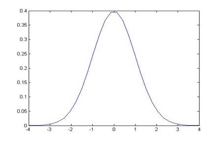
The area in blue is 5%; the area in the middle is 95%.

 

In the case of differences between those with a 4-year college degree and those with an advanced degree, this difference in time is 65.2511 – 70.0430 = -4.7919.  To find the standard error of the difference in means we first find the standard error of the first mean, which is 101.45307/sqrt(12388) = 0.9115; the standard error of the second mean is 103.82020/sqrt(5796) = 1.3637.  Therefore the standard error of the difference is sqrt(.9115^2 + 1.3637^2) = 1.6403.  Form a 95% confidence interval by using the reference value of 1.96.  Therefore a 95% confidence interval for the difference is -4.7919 ± (1.96 * 1.6403) = -4.7919 ± 3.2150 which is the interval (-8.0069,-1.5769).  Since this interval does not include zero, we can reject the null hypothesis of zero.

 

To review, we can reject, with 95% confidence, the null hypothesis of zero if the absolute value of the z-statistic is greater than 1.96,  where .  Re-arrange this to state that we reject if , which is equivalent to the statement that we can reject if .

 

To construct a 99% confidence interval, we'd have to find the Z that brackets 99% of the area under the standard normal – you should be able to do this.  Then use that number instead of 1.96.  For a 90% confidence interval, use a number that brackets 90% of the area and use that number instead of 1.96.

 

 

P-values

If confidence intervals weren't confusing enough, we can also construct equivalent hypothesis tests with p-values.  Where the Z-statistic tells how many standard errors away from zero is the observed difference (leaving it for us to know that more than 1.96 implies less than 5%), the p-value calculates this directly.  So a p-value for the difference above, between time spent by those with a college degree and those with an advanced degree, is found from -4.7919/1.6403 = -2.92.  So the area in the tail to the left of -2.92 is NORMSDIST(-2.92) = .0017; the area in both tails symmetrically is .0034.  The p-value for this difference is 0.34%; there is only a 0.34% chance that, if the true difference were zero, we could observe a number as big as -4.7919 in a sample of this size.

 

(Review: create a joint/marginal probability table showing educational qualifications and children.)

 

Confidence Intervals for Polls

I promised that I would explain to you how pollsters figure out the "±2 percentage points" margin of error for a political poll.  Now that you know about Confidence Intervals you should be able to figure these out.  Remember (or go back and look up) that for a binomial distribution the standard error is , where p is the proportion of "one" values and N is the number of respondents to the poll.  We can use our estimate of the proportion for p or, to be more conservative, use the maximum value of p(1 – p) where is p= ½.  A bit of quick math shows that with .  So a poll of 100 people has a maximum standard error of ; a poll of 400 people has maximum standard error half that size, of .025; 900 people give a maximum standard error 0.0167, etc. 

 

A 95% Confidence Interval is 1.96 (from the Standard Normal distribution) times the standard error; how many people do we need to poll, to get a margin of error of ±2 percentage points?  We want  so this is, at maximum where p= ½, 2401.

 

A polling organization therefore prices its polls depending on the client's desired accuracy: to get ±2 percentage points requires between 2000 and 2500 respondents; if the client is satisfied with just ±5 percentage points then the poll is cheaper.  (You can, and for practice should, calculate how many respondents are needed in order to get a margin of error of 2, 3, 4, and 5 percentage points.  For extra, figure that a pollster needs to only get the margin to ±2.49 percentage points in order to round to ±2, so they can get away with slightly fewer.)

 

 

Review

Take a moment to appreciate the amazing progress we've made: having determined that a sample average has a normal distribution, we are able to make a lot of statements about the probability that various hypotheses are true and about just how precise this measurement is.

 

What does it mean, "The sample average has a normal distribution"?  Now you're getting accustomed to this – means standardize into a Z-score, then lookup against a standard normal table.  But just consider how amazing this is.  For millennia, humans tried to say something about randomness but couldn't get much farther than, well, anything can happen – randomness is the absence of logical rules; sometimes you flip two heads in a row, sometimes heads and tails – who knows?!  People could allege that finding the sample average told something, but that was purely an allegation – unfounded and un-provable, until we had a normal distribution.  This normal distribution still lets "anything happen" but now it assigns probabilities; says that some outcomes are more likely than others.

 

And it's amazing that we can use mathematics to say anything useful about random chance.  Humans invented math and thought of it as a window into the unchanging eternal heavens, a glimpse of the mind of some god(s) – the Pythagoreans even made it their religion.  Math is eternal and universal and unchanging.  How could it possibly say anything useful about random outcomes?  But it does!  We can write down a mathematical function that describes the normal distribution; this mathematical function allows us to discover a great deal about the world and how it works.

 

Let's go back to this basic idea and re-visit an example I gave earlier, that the sample mean has a normal distribution.  I gave an example; let's do it again.

 

We've been working on the fraction of households with children; let's continue with that.  (This is atus_kids.xlsx.)  I used SPSS to "Save As" an Excel file, taking just the "has kids" dummy variable and the time spent with kids.   I want to treat the 98,778 people in the ATUS data as the population and show that small "polls" with just 100 people still get a pretty accurate measure of what fraction of people have kids.  In this case it's easy to find the true fraction of people with kids; if this were a real poll then cost would make it prohibitive to interview nearly 100,000 people so getting data from just 100 of them might be all that is possible.  In the Excel sheet, the tab for "Population" shows all of this data. 

 

The tab called "polls"  models these random polls.  A poll randomly selects a person from the population; I select one of the people in the population by choosing a random number between 1 and 98,778.  To do this, use RAND() to get a random number uniformly between zero and one.  Multiply it by 98,777 and use ROUND( ,0) to round that number to an integer.  This yields an integer between zero and 98777; add one to get a number between 1 and 98778.   Then I want a cell address so add one more.  This is the formula in cell C3, 2+ROUND(RAND()*98777,0).

 

To make Excel look up and deliver the value in this randomly-selected cell, use the text function CONCATENATE( )  which glues together textual values.  In this case I want to tell Excel to lookup in the "population" tab so this cell address is "population!" [the "!" alerts Excel that this is the name of a worksheet tab] and "A" to tell it column A.  So CONCATENATE("population!A",2+ROUND(RAND()*98777,0)) gives answers like "population!A45035".  (You are encouraged to take these formulas apart for yourself, to see how they work individually.)

 

Finally the INDIRECT( ) command tells Excel to lookup and deliver the value of the cell that is referenced, so this goes to the population, finds the 45,035^th observation (or another randomly chosen one) and yields "0".  Then each row is a poll; copy this cell across 100 columns to make a poll of 100 people.  But this is only one poll!  What if we did a different poll?  Copy the first row into another row for poll #2.  And another, and another – 1000 times.  This shows 1000 possible polls that could have been done.  Copy and paste these ("Paste As ... Values" to snip them as numbers) to the next sheet.  Do this a few times to get a few thousand.  Plot a histogram – see?! It's Normal!