SPSS Examples

Econ 29000, Principles of Statistics

Kevin R Foster, CCNY

Spring 2011

Hypothesis Tests

Using the ATUS data, we want to compare the amount of time people spend with kids.

So load the ATUS dataset into SPSS to begin with a screen like this:

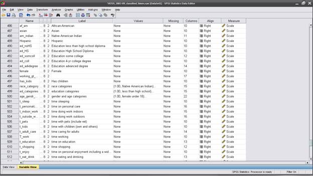
That just shows the data.

Run the syntax file that I gave, "classification.sps" – "File \ Open \ Syntax " to get this:

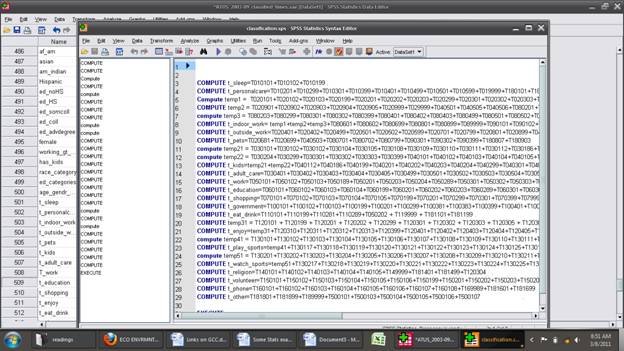
Then "Run \ All" from that menu.

This creates some broad classifications – you could make your own but for now this allows us to all be looking at the data in the same way.

One of the created variables is "t_kids" the time spent with children (either household's children or non-household children).

We will look at how education levels change the amount of time people spend with their children. There are two separate decisions that change this time: first, does the household have any children at all; second, if they have kids, how much time do they spend?

Begin by looking at the first: what fraction have kids? We want to know, of households that could have kids, what fraction have them? This "of households that could have kids" is important since we know that elderly people are unlikely to have kids (although it can happen; they might have custody of grandchildren). But it's plausible to restrict the analysis to just people from, say, 20-50 years old.

So "Data \ Select Cases" brings this screen:

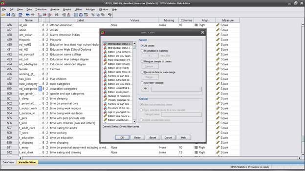
And click "If Condition is Satisfied" and the button for "If ..." to bring up this screen:

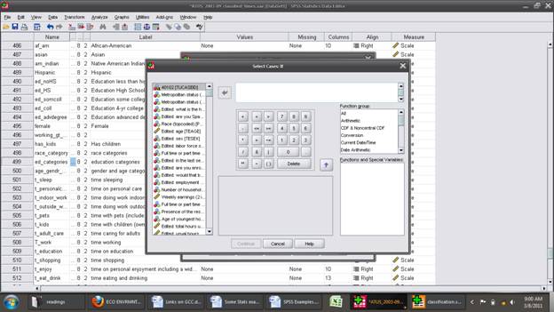
Type and/or use the buttons to create " (TEAGE > 20) & (TEAGE < 50)" to select people in the 20-50 year old group. (Could use >= and <=; you could argue for different age ranges; all of these variations can be explored by you later.) Click "Continue" and then "OK" and SPSS will display some output verifying that this was done.

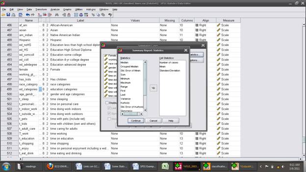
Now I will use "Analyze \ Descriptive Statistics \ Explore" (shortcut is discussed below). The "Dependent List" is "has_kids" and the "Factor List" is "education categories". (I choose the radio button at the bottom to just display "Statistics" not "Plots" but this is just my choice.)

This gives this output:

EXAMINE VARIABLES=has_kids BY ed_categories /PLOT NONE /STATISTICS DESCRIPTIVES /CINTERVAL 95 /MISSING LISTWISE /NOTOTAL.

Explore

education categories

Case Processing Summary
	education categories	Cases
		Valid		Missing		Total
		N	Percent	N	Percent	N	Percent
Has children	less than high school	4700	100.0%	0	.0%	4700	100.0%
	high school diploma	13223	100.0%	0	.0%	13223	100.0%
	some college	15465	100.0%	0	.0%	15465	100.0%
	college degree	12388	100.0%	0	.0%	12388	100.0%
	advanced degree	5796	100.0%	0	.0%	5796	100.0%

Descriptives
	education categories			Statistic	Std. Error
Has children	less than high school	Mean		.7377	.00642
		95% Confidence Interval for Mean	Lower Bound	.7251
			Upper Bound	.7502
		5% Trimmed Mean		.7641
		Median		1.0000
		Variance		.194
		Std. Deviation		.43995
		Minimum		.00
		Maximum		1.00
		Range		1.00
		Interquartile Range		1.00
		Skewness		-1.081	.036
		Kurtosis		-.832	.071
	high school diploma	Mean		.6936	.00401
		95% Confidence Interval for Mean	Lower Bound	.6858
			Upper Bound	.7015
		5% Trimmed Mean		.7152
		Median		1.0000
		Variance		.213
		Std. Deviation		.46100
		Minimum		.00
		Maximum		1.00
		Range		1.00
		Interquartile Range		1.00
		Skewness		-.840	.021
		Kurtosis		-1.294	.043
	some college	Mean		.6779	.00376
		95% Confidence Interval for Mean	Lower Bound	.6705
			Upper Bound	.6852
		5% Trimmed Mean		.6976
		Median		1.0000
		Variance		.218
		Std. Deviation		.46731
		Minimum		.00
		Maximum		1.00
		Range		1.00
		Interquartile Range		1.00
		Skewness		-.761	.020
		Kurtosis		-1.421	.039
	college degree	Mean		.6606	.00425
		95% Confidence Interval for Mean	Lower Bound	.6522
			Upper Bound	.6689
		5% Trimmed Mean		.6784
		Median		1.0000
		Variance		.224
		Std. Deviation		.47354
		Minimum		.00
		Maximum		1.00
		Range		1.00
		Interquartile Range		1.00
		Skewness		-.678	.022
		Kurtosis		-1.540	.044
	advanced degree	Mean		.6839	.00611
		95% Confidence Interval for Mean	Lower Bound	.6719
			Upper Bound	.6959
		5% Trimmed Mean		.7044
		Median		1.0000
		Variance		.216
		Std. Deviation		.46498
		Minimum		.00
		Maximum		1.00
		Range		1.00
		Interquartile Range		1.00
		Skewness		-.791	.032
Kurtosis		-1.374	.064

Which is rather long because it gives us so many measures! We might want a bit of a shortcut, once we figure out which measures we're truly interested in.

So use "Analyze \ Reports \ Case Summaries" and put "has_kids" into "Variables" and "education_categories" into "Grouping Variable(s)". Un-check "Display Cases" and click "Statistics" to choose Number of Cases, Mean, and Standard Deviation.

Then "Continue" then,

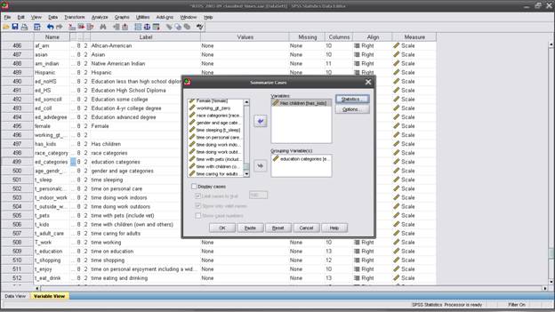
"OK" which will run and give this output:

Summarize

Case Processing Summary
	Cases
	Included		Excluded		Total
	N	Percent	N	Percent	N	Percent
Has children * education categories	51572	100.0%	0	.0%	51572	100.0%

Case Summaries
Has children
education categories	N	Mean	Std. Deviation
less than high school	4700	.7377	.43995
high school diploma	13223	.6936	.46100
some college	15465	.6779	.46731
college degree	12388	.6606	.47354
advanced degree	5796	.6839	.46498
Total	51572	.6839	.46497

Which is much easier to read. From either output, we can see that 74% of people who are 20-50 years old have kids, 69% of people with a high-school diploma, 68% with some college, etc.

We want to test: is the fraction of people with kids different by educational qualification? Is 74% a "big" difference from 69%, or could it just be due to random error?

For this simple test we find the difference is 0.7377 – 0.6936 = 0.0441. To find the standard error of this difference in means, we first find the standard error of each mean, which is 0.43995/sqrt(4700) = 0.006417 and 0.46100/sqrt(13223) = 0.004009. To find the standard error of the difference in means, square each standard error, add them, and take the square root. With (where se(A) is the standard error of the average of A, σ_A is the standard deviation of the sample A, and N_A is the number of observations in sample A) and analogously , find the standard error of the difference as = 0.007567.

So find the Z-statistic, the standardized value of the difference in the means, as the actual difference, 0.0441, minus the difference hypothesized by the null (which is zer0), divided by its standard error, so = 5.83.

What is the probability, that the true value is zero, and I could observe a value as large (in absolute value) as 5.83? The area in the tails beyond 5.83 is, from taking a look at the graph,

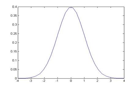
really tiny since 5.83 is off the edge of the picture. Use Excel to find that this is 0.000000006 – which is zero, if rounded to 3 or 4 decimal places. So there is essentially a zero probability that there could actually be no difference, yet we would observe a 3 percentage point difference in the data. We reject the null hypothesis that there is no difference; the data allow us to conclude that there is a big difference.

You can and should be able to do the rest of the tests for the other educational categorizations.

Now run the Case Summary with "t_kids" instead of just has kids, and find

Case Summaries
time with children (own and others)
education categories	N	Mean	Std. Deviation
less than high school	4700	47.6104	94.33761
high school diploma	13223	48.9654	89.57632
some college	15465	53.9291	93.87316
college degree	12388	65.2511	101.45307
advanced degree	5796	70.0430	103.82020
Total	51572	56.6112	96.21166

Now we see a steady rise, that people with more education spend more time with kids. Again we can ask if these difference are significant: is the mean for "less than high school" a big difference from mean for "high school diploma"?

Again find the Z-score. The difference is 47.6104 – 48.9654 = -1.355. The standard error of the first is 94.33761/sqrt(4700) = 1.376; the standard error of the second is 89.57632/sqrt(13223) = 0.779. The standard error of the difference is sqrt( 1.376² + 0.779²) = 1.581. So the Z-score of the difference in time is -1.355/1.581 = -.857.

What is now the probability, if there were actually no difference, of seeing a Z-score as large (in absolute value) as -0.857? This is the area in the tails farther from zero than ±0.857,

Which, from NORMSDIST(-0.857), has .196 area in the left tail and an equivalent area in the right, so the overall probability is 0.392 – almost a 40% chance of seeing such a difference, if there were actually zero difference. So we do not reject the null hypothesis – we cannot conclude that there is a big difference.

You can and should do those tests for the other classifications. Note that you can do lots of pairwise comparisons (no HS vs advanced degree) and so you might end up worrying if this is really fair (we'll get to that; it's not quite right). You could also use other scales such as the differences as a percent change – a 1.4 minute difference doesn't sound big but 1.355/47.6 is a 2.8% difference (or calculate that 1.4 minutes per day is about 8.25 hours per year; or if we figure about 14% of the US population of 300m is in this category, then this could be blown up to nearly 40,000 years – which makes the statistic sound terrifying! (A reminder about how to lie with statistics.)

Then the interesting further question becomes: if higher-education households spend more time with kids, what are they doing less of – i.e. how do they manage it? Is this less time spent doing chores (maybe hiring someone to do these)? Alternately, is this a story of gender – do less-educated men spend less time with kids, in a more traditional gender role? You can pursue these questions for yourself.