Past Exam Questions

Econ 29000

Kevin R Foster, CCNY

Spring 2011

Not all of these questions are strictly relevant; some might require a bit of knowledge that we haven't covered this year, but they're a generally good guide.

1. (20 points) A random variable is distributed as a standard normal. (You are encouraged to sketch the PDF in each case.)

a. (5 points) What is the probability that we could observe a value as far or farther than 1.3?

b. (5 points) What is the probability that we could observe a value nearer than 1.8?

c. (5 points) What value would leave 10% of the probability in the right-hand tail?

d. (5 points) What value would leave 25% in both the tails (together)?

2. (20 points) Using the CPS 2010 data (on Blackboard, although you don't need to download it for this), restricting attention to only those reporting a non-zero wage and salary, the following regression output is obtained for a regression (including industry, occupation, and state fixed effects) with wage and salary as the dependent variable.

a. (14 points) Fill in the missing values in the table.

b. (3 points) The dummy variables for veterans have been split into various time periods to distinguish recent veterans from those who served decades ago. If you knew that the draft ended at about the same time as the Vietnam war, how would that affect your interpretation of the coefficient estimates?

c. (3 points) Critique the regression: how would you improve the estimates (using the same dataset)?

ANOVA^b
Model		Sum of Squares	df	Mean Square	F	Sig.
1	Regression	8.201E+13	152	5.395E+11	324.098	.000^a
	Residual	1.639E+14	98479	1.665E+09
	Total	2.460E+14	98631

Coefficients^a
Model		Unstandardized Coefficients		Standardized Coefficients	t	Sig.
		B	Std. Error	Beta
1	(Constant)	12970.923	2290.740		5.662	.000
	Demographics, Age	2210.038	62.066	.605	____	____
	Age squared	-21.527	.693	-.504	____	____
	Female	-14892.950	____	-.149	-47.872	.000
	African American	-3488.065	____	-.022	-7.809	.000
	Asian	-2700.032	____	-.012	-2.782	.005
	Native American Indian or Alaskan or Hawaiian	____	824.886	-.009	-3.442	.001
	Hispanic	____	483.313	-.024	-6.847	.000
	Immigrant	____	632.573	-.032	-6.728	.000
	1 or more parents were immigrants	989.451	541.866	.008	____	____
	immig_india	-456.482	1675.840	-.001	____	____
	immig_SEAsia	821.730	1252.853	.003	____	____
	immig_MidE	-599.852	2335.868	-.001	____	____
	immig_China	3425.017	1821.204	.006	____	____
	Education: High School Diploma	2786.569	492.533	.025	5.658	.000
	Education: Some College but no degree	5243.544	528.563	.042	9.920	.000
	Education: Associate in vocational	6530.542	762.525	.028	8.564	.000
	Education: Associate in academic	7205.474	736.838	.032	9.779	.000
	Education: 4-yr degree	17766.941	576.905	.143	30.797	.000
	Education: Advanced Degree	36755.485	703.658	.227	52.235	.000
	Married	4203.602	414.288	.042	10.147	.000
	Divorced or Widowed or Separated	830.032	501.026	.006	1.657	.098
	kids_under18	3562.643	327.103	.036	10.891	.000
	kids_under6	-721.123	404.818	-.006	-1.781	.075
	Union member	4868.240	976.338	.013	4.986	.000
	Veteran since Sept 2001	2081.909	4336.647	.001	.480	.631
	Veteran Aug 1990 - Aug 2001	-1200.688	1788.034	-.002	-.672	.502
	Veteran May 1975-July 1990	-1078.953	1895.197	-.001	-.569	.569
	Veteran August 1964-April 1975	-6377.461	3195.784	-.005	-1.996	.046
	Veteran Feb 1955-July 1964	-7836.420	4904.511	-.004	-1.598	.110
	Veteran July 1950-Jan 1955	-19976.382	10570.869	-.005	-1.890	.059
	Veteran before 1950	-15822.026	12943.766	-.003	-1.222	.222

3. (25 points) Using the NHANES 2007-09 data (on Blackboard, although you only need to download it for the very last part), reporting a variety of socioeconomic variables as well as behavior choices such as the number of sexual partners reported (number_partners), we want to see if richer people have more sex than poor people. The following table is constructed, showing three categories of family income and 5 categories of number of sex partners:

	number of sex partners
family income	zero	1	2 - 5	6 - 25	>25	Marginal:
< 20,000	11	63	236	255	92	______
20 - 45,000	7	117	323	308	117	______
> 45,000	3	234	517	607	218	______
Marginal:	______	______	______	______	______

a. (5 points) Where is the median, for number of sex partners, for poorer people? For middle-income people? For richer people?

b. (5 points) Conditional on a person being poorer, what is the likelihood that they report fewer than 6 partners? Conditional on being middle-income? Richer?

c. (5 points) Conditional on reporting 2-5 sex partners, what is the likelihood that a person is poorer? Middle-income? Richer?

d. (5 points) Explain why the average number of sex partners might not be as useful a measure as, for example, the data ranges above or the median or the 95%-trimmed mean.

e. (5 points) (You will need to download the data for this part) Could the difference be explained by schooling effects? How does college affect the number of sex partners?

4. (15 points) I provide a dataset online (stock_indexes.sav on Blackboard) with the daily returns on the S&P 500 stock index and its daily returns as well as the NASDAQ index and its returns, from January 1, 1980 to December 9, 2010.

a. (5 points) What is the mean and standard deviation?

b. (5 points) If the stock index returns were distributed normally, what value of return is low enough, that 95% of the days are better?

c. (5 points) What is the 5% value of the actual returns (the fifth percentile, use "Analyze\Descriptive Statistics\Explore" and check "Percentiles" in "Options")? Is this different from your previous answer? What does that imply? Explain.

5. (25 points) Using the CPS 2010 data online, examine whether children are covered by Medicaid or other insurance plan. Run a crosstab on "CH_HI" whether a child has health insurance, and "CH_MC" if a child is covered by Medicaid.

a. (10 points) What fraction of children are covered by Medicaid? What fraction of children are not covered by any policy?

b. (15 points) What is the average family income of children who are covered by Medicaid? Of children who are not? What is the t-statistic and p-value for a statistical test of whether the means are equal?

6. (15 points) The oil and gas price dataset online, (oil_gas_prices.sav on Blackboard, although you only need to download it for the very last part), has data on prices of oil, gasoline, and heating oil (futures prices, in this case). Compare two regression specifications of the current price of gasoline. Specification A explains the current price with its price the day before. Specification B has the price of gas on the day before but also includes the prices of crude oil and heating oil on the day before. The estimates of the coefficient on gasoline are shown below:

	Coefficient estimate	Standard error
Specification A	0.021	0.028
Specification B	0.153	0.048

a. (5 points) Calculate t-statistics and p-values for each specification of the regression.

b. (5 points) Explain what you could learn from each of these regressions – specifically, would it be a good idea to invest in gasoline futures?

c. (5 points) Explain why there is a difference in the estimated coefficients. Can you say that one is more correct?

7. (20 Points) A random variable is distributed as a standard normal. (You are encouraged to sketch the PDF in each case.)

a. (5 points) What is the probability that we could observe a value as far or farther than -0.9?

b. (5 points) What is the probability that we could observe a value nearer than 1.4?

c. (5 points) What value would leave 5% of the probability in the right-hand tail?

d. (5 points) What value would leave 5% in both the tails (together)?

8. [this question was given in advance for students to prepare with their group} Download (from Blackboard) and prepare the dataset on the 2004 Survey of Consumer Finances from the Federal Reserve. Estimate the probability that each head of household (restrict to only heads of household!) has at least one credit card. Write up a report that explains your results (you might compare different specifications, you might consider different sets of socioeconomic variables, different interactions, different polynomials, different sets of fixed effects, etc.).

9. Explain in greater detail your topic for the final project. Include details about the dataset which you will use and the regressions that you will estimate. Cite at least one previous study which has been done on that topic (published in a refereed journal).

10. You want to examine the impact of higher crude oil prices on American driving habits during the past oil price spike. A regression of US gasoline purchases on the price of crude oil as well as oil futures gives the coefficients below. Critique the regression and explain whether the necessary basic assumptions hold. Interpret each coefficient; explain its meaning and significance.

Coefficients(a)

Model		Unstandardized Coefficients		Standardized Coefficients	t	Sig.
		B	Std. Error	Beta
1	(Constant)	.252	.167		1.507	.134
	return on crude futures, 1 month ahead	.961	.099	.961	9.706	.000
	return on crude futures, 2 months ahead	-.172	.369	-.159	-.466	.642
	return on crude futures, 3 months ahead	.578	.668	.509	.864	.389
	return on crude futures, 4 months ahead	-.397	.403	-.333	-.986	.326
	US gasoline consumption	-.178	.117	-.036	-1.515	.132
	Spot Price Crude Oil Cushing, OK WTI FOB (Dollars per Barrel)	4.23E-005	.000	.042	1.771	.079

a Dependent Variable: return on crude spot price

11. You estimate the following coefficients for a regression explaining log individual incomes:

Coefficients(a)

Model		Unstandardized Coefficients		Standardized Coefficients	t	Sig.
		B	Std. Error	Beta	B	Std. Error
1	(Constant)	6.197	.026		239.273	.000
	Demographics, Age	.154	.001	1.769	114.120	.000
	agesq	-.002	.000	-1.594	-107.860	.000
	female	-.438	.017	-.184	-25.670	.000
	afam	-.006	.010	-.002	-.590	.555
	asian	-.011	.015	-.002	-.713	.476
	Amindian	-.063	.018	-.009	-3.573	.000
	Hispanic	.053	.010	.016	5.139	.000
	ed_hs	.597	.014	.226	43.251	.000
	ed_smcol	.710	.014	.272	50.150	.000
	ed_coll	1.138	.015	.379	74.378	.000
	ed_adv	1.388	.018	.355	78.917	.000
	Married	.222	.009	.092	25.579	.000
	Divorced Widowed Separated	.138	.011	.041	12.311	.000
	union	.189	.021	.022	8.951	.000
	veteran	.020	.012	.004	1.646	.100
	immigrant	-.055	.013	-.017	-4.116	.000
	2^nd Generation Immigrant	.064	.012	.022	5.268	.000
	female*ed_hs	-.060	.020	-.017	-2.948	.003
	female*ed_smcol	-.005	.020	-.002	-.270	.787
	female*ed_coll	-.104	.022	-.026	-4.806	.000
	female*ed_adv	-.056	.025	-.010	-2.218	.027

a Dependent Variable: lnwage

a. Explain your interpretation of the final four coefficients in the table.

b. How would you test their significance? If this test got "Sig. = 0.13" from SPSS, interpret the result.

c. What variables are missing? Explain how this might affect the analysis.

12. You are in charge of polling for a political campaign. You have commissioned a poll of 300 likely voters. Since voters are divided into three distinct geographical groups, the poll is subdivided into three groups with 100 people each. The poll results are as follows:

	total	A	B	C
number in favor of candidate	170	58	57	55
number total	300	100	100	100
std. dev. of poll	0.4956	0.4936	0.4951	0.4975

Note that the standard deviation of the sample (not the standard error of the average) is given.

d. Calculate a t-statistic, p-value, and a confidence interval for the main poll (with all of the people) and for each of the sub-groups.

e. In simple language (less than 150 words), explain what the poll means and how much confidence the campaign can put in the numbers.

f. Again in simple language (less than 150 words), answer the opposing candidate's complaint, "The biased media confidently says that I'll lose even though they admit that they can't be sure about any of the subgroups! That's neither fair nor accurate!"

13. Fill in the blanks in the following table showing SPSS regression output. The model has the dependent variable as time spent working at main job.

Coefficients(a)

Model		Unstandardized Coefficients		Standardized Coefficients	t	Sig.
		B	Std. Error	Beta
1	(Constant)	198.987	7.556		26.336	.000
	female	-65.559	4.031	-.138	___?___	___?___
	African-American	-9.190	6.190	-.013	___?___	___?___
	Hispanic	17.283	6.387	.024	___?___	___?___
	Asian	1.157	12.137	.001	___?___	___?___
	Native American/Alaskan Native	-28.354	14.018	-.017	-2.023	.043
	Education: High School Diploma	___?___	6.296	.140	11.706	.000
	Education: Some College	___?___	6.308	.174	14.651	.000
	Education: 4-year College Degree	110.064	___?___	.183	16.015	.000
	Education: Advanced degree	126.543	___?___	.166	15.714	.000
	Age	-1.907	___?___	-.142	-16.428	.000

a Dependent Variable: Time Working at main job

14. Suppose I were to start a hedge fund, called KevinNeedsMoney Limited Ventures, and I want to present evidence about how my fund did in the past. I have data on my fund's returns, Ret_t, at each time period t, and the returns on the market, Mkt_t. The graph below shows the relationship of these two variables:

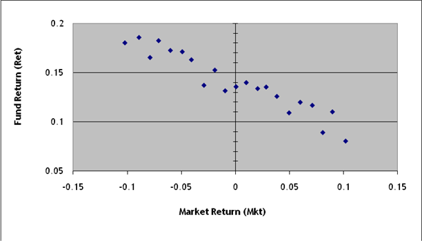
a. I run a univariate OLS regression, . Approximately what value would be estimated for the intercept term, b₀? For the slope term, b₁?

b. How would you describe this fund's performance, in non-technical language – for instance if you were advising a retail investor without much finance background?

15. Using the American Time Use Study (ATUS) we measure the amount of time that each person reported that they slept. We run a regression to attempt to determine the important factors, particularly to understand whether richer people sleep more (is sleep a normal or inferior good) and how sleep is affected by labor force participation. The SPSS output is below.

Coefficients(a)
Model		Unstandardized Coefficients		Standardized Coefficients
		B	Std. Error	Beta	t	Sig.
1	(Constant)	-4.0717	4.6121		-0.883	0.377
	female	23.6886	1.1551	0.18233	20.508	0.000
	African-American	-8.5701	1.7136	-0.04369	-5.001	0.000
	Hispanic	10.1015	1.7763	0.05132	5.687	0.000
	Asian	-1.9768	3.3509	-0.00510	-0.590	0.555
	Native American/Alaskan Native	-3.5777	3.8695	-0.00792	-0.925	0.355
	Education: High School Diploma	2.5587	1.8529	0.01768	1.381	0.167
	Education: Some College	-0.3234	1.8760	-0.00222	-0.172	0.863
	Education: 4-year College Degree	-1.3564	2.0997	-0.00821	-0.646	0.518
	Education: Advanced degree	-3.3303	2.4595	-0.01590	-1.354	0.176
	Weekly Earnings	0.000003	0.000012	-0.00277	-0.246	0.806
	Number of children under 18	2.0776	0.5317	0.03803	3.907	0.000
	person is in the labor force	-11.6706	1.7120	-0.08401	-6.817	0.000
	has multiple jobs	0.4750	2.2325	0.00185	0.213	0.832
	works part time	4.2267	1.8135	0.02244	2.331	0.020
	in school	-5.4641	2.2993	-0.02509	-2.376	0.017
	Age	1.1549	0.1974	0.31468	5.850	0.000
	Age-squared	-0.0123	0.0020	-0.33073	-6.181	0.000

a. Which variables are statistically significant at the 5% level? At the 1% level?

b. How much more or less time (in minutes) would be spent sleeping by a male college graduate who is African-American and working full-time, bringing weekly earnings of $1000?

c. Are there other variables that you think are important and should be included in the regression? What are they, and why?

16. You are given the following output from a logit regression using ATUS data. The dependent variable is whether the person spent any time cleaning in the kitchen and the independent variables are the usual list of race/ethnicity (African-American, Asian, Native American, Hispanic), female, educational attainment (high school diploma, some college, a 4-year degree, or an advanced degree), weekly earnings, the number of kids in the household, dummies if the person is in the labor force, has multiple jobs, works part-time, or is in school now, as well as age and age-squared. We include a dummy if there is a spouse or partner present and then an interaction term for if the person is male AND there is a spouse in the household. There are only adults in the sample. Descriptive statistics show that approximately 5% of men clean in the kitchen while 20% of women do. The SPSS output for the logit regression is:

	B	S.E.	Wald	df	Sig.	Exp(B)
female	0.9458	0.0860	120.945	1	0.000	2.5749
African-American	-0.6113	0.0789	60.079	1	0.000	0.5427
Hispanic	-0.2286	0.0765	8.926	1	0.003	0.7956
Asian	0.0053	0.1360	0.001	1	0.969	1.0053
Native American	-0.0940	0.1618	0.338	1	0.561	0.9103
Education: high school	0.0082	0.0789	0.011	1	0.917	1.0082
Education: some college	0.0057	0.0813	0.005	1	0.944	1.0057
Education: college degree	0.0893	0.0887	1.013	1	0.314	1.0934
Education: advanced degree	0.0874	0.1009	0.751	1	0.386	1.0914
Weekly Earnings	0.0000007	0.0000005	1.943	1	0.163	1.0000
Num. Kids in Household	0.2586	0.0226	131.473	1	0.000	1.2952
person in the labor force	-0.5194	0.0694	55.967	1	0.000	0.5949
works multiple jobs	-0.2307	0.1009	5.223	1	0.022	0.7940
works part-time	0.1814	0.0733	6.130	1	0.013	1.1989
person is in school	-0.1842	0.1130	2.658	1	0.103	0.8318
Age	0.0551	0.0088	38.893	1	0.000	1.0567
Age-squared	-0.0004	0.0001	22.107	1	0.000	0.9996
spouse is present	0.5027	0.0569	78.074	1	0.000	1.6531
Male * spouse is present	-0.6562	0.1087	36.462	1	0.000	0.5188
Constant	-3.3772	0.2317	212.434	1	0.000	0.0341

a. Which variables from the logit are statistically significant at the 5% level? At the 1% level?

b. How would you interpret the coefficient on the Male * spouse-present interaction term? What is the age when a person hits the peak probability of cleaning?

17. Use the SPSS dataset, atus_tv from Blackboard, which is a subset of the American Time Use survey. This time we want to find out which factors are important in explaining whether people spend time watching TV. There are a wide number of possible factors that influence this choice.

a. What fraction of the sample spend any time watching TV? Can you find sub-groups that are significantly different?

b. Estimate a regression model that incorporates the important factors that influence TV viewing. Incorporate at least one non-linear or interaction term. Show the SPSS output. Explain which variables are significant (if any). Give a short explanation of the important results.

18. This question refers to your final project.

g. What data set will you use?

h. What regression (or regressions) will you run? Explain carefully whether the dependent variable is continuous or a dummy, and what this means for the regression specification. What independent variables will you include? Will you use nonlinear specifications of any of these? Would you expect heteroskedasticity?

i. What other variables are important, but are not measured and available in your data set? How do these affect your analysis?

19. Estimate the following regression:: S&P100 returns = b₀ + b₁(lag S&P100 returns) + b₂(lag interest rates) + ε

using the dataset, financials.sav. Explain which coefficients (if any) are significant and interpret them.

20. A study by Mehran and Tracy examined the relationship between stock option grants and measures of the company's performance. They estimated the following specification:

Options = b₀+b₁(Return on Assets)+b₂(Employment)+b₃(Assets)+b₄(Loss)+u

where the variable (Loss) is a dummy variable for whether the firm had negative profits. They estimated the following coefficients:

	Coefficient	Standard Error
Return on Assets	-34.4	4.7
Employment	3.3	15.5
Assets	343.1	221.8
Loss Dummy	24.2	5.0

Which estimate has the highest t-statistic (in absolute value)? Which has the lowest p-value? Show your calculations. How would you explain the estimate on the "Loss" dummy variable?

21. A paper by Farber examined the choices of how many hours a taxidriver would work, depending on a number of variables. His output is:

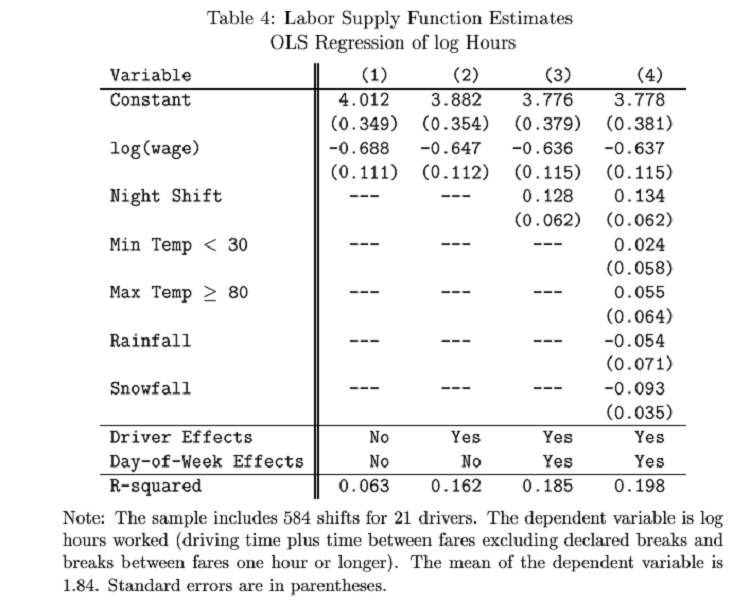
"Driver Effects" are fixed effects for the 21 different drivers.

a. What is the estimated elasticity of hours with respect to the wage?

b. Is there a significant change in hours on rainy days? On snowy days?

22. A paper by Gruber looks at the effects of divorce on children (once they become adults), including whether there was an increase or decrease in education and wages. Gruber uses data on state divorce laws: over time some states changed their laws to make divorce easier (no-fault or unilateral divorce). Why do you think that he used state-level laws rather than the individual information (which was in the dataset) about whether a person's parents were divorced? Is it important that he documents that states with easier divorce laws had more divorces? If he ran a regression that explained an adult's wage on the usual variables, plus a measure of whether that person's parents had been divorced, what complications might arise? Explain.

23. (20 points) Using the data on New Yorkers in 1910, we estimate a binary logistic (logit) model to explain labor force participation (whether each person was working for pay) as a function of gender (a dummy variable for female), race (a dummy for African-American), nativity (a dummy if the person is an immigrant and then another dummy if they are second-generation – their parents were immigrants), marital status (three dummies: one for married; one for Divorced/Separated; one for Widow(er)s), age, age-squared, and interaction effects. We allow interactions between Female and Married (fem_marr = Married * Female), and then between Age and Immigrant (age_immig = Age * Immigrant) and Age-Squared and Immigrant (agesq_immig = Age² * Immigrant). Explain the following regression results:

Variables in the Equation

		B	S.E.	Wald	df	Sig.	Exp(B)
Step 1(a)	female	-1.890	.122	240.805	1	.000	.151
	AfricanAmer	2.703	.235	132.625	1	.000	14.919
	Married	1.144	.193	35.245	1	.000	3.141
	fem_marr	-4.946	.209	562.000	1	.000	.007
	DivSep	.251	.568	.195	1	.658	1.285
	Widow	-1.238	.131	89.790	1	.000	.290
	immigrant	1.575	1.167	1.822	1	.177	4.831
	immig2g	.068	.117	.338	1	.561	1.070
	Age	.114	.047	5.858	1	.016	1.121
	age_sqr	-.00176	.001	7.137	1	.008	.998
	age_immig	-.035	.068	.263	1	.608	.966
	agesq_immig	0.00027	.001	.080	1	.777	1.000
	Constant	1.069	.795	1.809	1	.179	2.911

a Variable(s) entered on step 1: female, AfricanAmer, Married, fem_marr, DivSep, Widow, immigrant, immig2g, age, age_sqr, age_immig, agesq_immig.

At what age do natives peak in their labor force participation? Immigrants? Which is higher? The regression shows that women are less likely to be in the labor force, married people are more likely, African-Americans are more likely, and immigrants are more likely to be in the labor force. Interpret the coefficient on the female-married interaction.

24. (15 points) Calculate the probability in the following areas under the Normal pdf with mean and standard deviation as given. You might usefully draw pictures as well as making the calculations. For the calculations you can use either a computer or a table.

a. What is the probability, if the true distribution has mean -15 and standard deviation of 9.7, of seeing a deviation as large (in absolute value) as -1?

b. What is the probability, if the true distribution has mean 0.35 and standard deviation of 0.16, of seeing a deviation as large (in absolute value) as 0.51?

c. What is the probability, if the true distribution has mean -0.1 and standard deviation of 0.04, of seeing a deviation as large (in absolute value) as -0.16?

25. (20 points) Using data from the NHIS, we find the fraction of children who are female, who are Hispanic, and who are African-American, for two separate groups: those with and those without health insurance. Compute tests of whether the differences in the means are significant; explain what the tests tell us. (Note that the numbers in parentheses are the standard deviations.)

	with health insurance	without health insurance
female	0.4905 (0.49994) N=7865	0.4811 (0.49990) N=950
Hispanic	0.2587 (0.43797) N=7865	0.5411 (0.49857) N=950
African American	0.1785 (0.38297) N=7865	0.1516 (0.35880) N=950

26. (25 points) Explain the topic of your final project. Carefully explain one regression that you are going to estimate (or have already estimated). Tell the dependent variable and list the independent variables. What hypothesis tests are you particularly interested in? What problems might arise in the estimation? Is there likely to be heteroskedasticity? Is it clear that the X-variables cause the Y-variable and not vice versa? Explain. [Note: these answers should be given in the form of well-written paragraphs not a series of bullet items answering my questions!]

27. (20 points) In estimating how much choice of college major affects income, Hamermesh & Donald (2008) send out surveys to college alumni. They first estimate the probability that a person will answer the survey with a probit model. They use data on major (school of education is the omitted category), how long ago the person graduated, and some information from their college record. Their results are (assume that the ₀ coefficient is 0.253):

		pr(respond to survey)	t-statistic
Major (Dummy variable)	Architecture and Fine Arts	-0.044	1.61
	Business---general	0.046	1.72
	Business---quantitative	0.038	1.45
	Communications	0.023	1.00
	Engineering	0.086	2.51
	Humanities	-0.013	0.54
	"Honors"	0.087	2.08
	Social Sciences	0.052	2.28
	Natural Sciences, Pharmacology	0.04	1.52
	Nursing, Social Work	0.061	1.57
dummy variables	Class of 1980	0.025	1.61
	Class of 1985	-0.009	0.61
	Class of 1990	0.041	2.65
	Class of 1995	0.033	2.20
	GPA	0.027	2.59
	Upper Div. Sci. & Math Credits	0.0001	0.21
	Upper Div. Sci. & Math Grades	0.002	0.51
	HS Area Income ($000)	0.001	1.92
	Female	0.031	3.06

What is the probability of reply for a major in quantitative Business, from the Class of 1995, with a GPA of 3.1, with 31 upper-division Science & Math credits, with a 2.9 GPA within those upper-division Science & Math courses, from a high school with a 40 HS Area Income? How much more or less is the probability, if the respondent is female?

28. (15 points) Consider the following regression output, from a regression of log-earnings on a variety of socioeconomic factors. Fill in the blanks in the "Coefficients" table. Then calculate the predicted change in the dependent variable when Age increases from 25 to 26; then when Age changes from 55 to 56 (note that Age_exp2 is Age² and Age_exp3 is Age³).

Model Summary

Model	R	R Square	Adjusted R Square	Std. Error of the Estimate
1	.613	.376	.376	.94098

ANOVA

Model		Sum of Squares	df	Mean Square	F	Sig.
1	Regression	53551.873	26	2059.687	2326.152	.000(a)
	Residual	88995.531	100509	.885
	Total	142547.403	100535

Coefficients(a)

Model		Unstandardized Coefficients		Standardized Coefficients	t	Sig.
		B	Std. Error	Beta
	(Constant)	3.841	0.059		65.581	0.000
	Education: High School Diploma	0.106	0.008	0.040305	__?__	__?__	ß
	Education: AS vocational	__?__	0.015	0.051999	19.644	0.000	ß
	Education: AS academic	0.344	__?__	0.062527	23.574	0.000	ß
	Education: 4 year College Degree	0.587	0.009	0.195326	65.257	0.000
	Education: Advanced Degree	0.865	0.011	0.221309	77.658	0.000
	geog2	0.070	0.013	0.017072	5.220	0.000
	geog3	0.005	0.013	0.001232	__?__	__?__	ß
	geog4	-0.050	0.013	-0.01345	__?__	__?__	ß
	geog5	0.062	0.012	0.019974	__?__	__?__	ß
	geog6	-0.061	0.017	-0.01039	__?__	__?__	ß
	geog7	0.026	0.014	0.006106	__?__	__?__	ß
	geog8	0.056	0.013	0.014445	4.303	0.000
	geog9	0.102	0.012	0.030892	8.357	0.000
	Married	__?__	0.009	0.062911	17.213	0.000	ß
	Widowed	__?__	0.025	-0.00191	-0.697	__?__	ß
	Divorced or Separated	__?__	0.012	0.022796	7.042	0.000	ß
	female	__?__	0.006	-0.19408	-76.899	0.000	ß
	union	0.208	__?__	0.024531	9.808	0.000	ß
	hispanic	-0.106	__?__	-0.03211	-12.012	0.000	ß
	Af_Amer	-0.038	__?__	-0.00995	-3.774	0.000	ß
	NativAm	-0.100	__?__	-0.01342	-5.322	0.000	ß
	AsianAm	-0.061	__?__	-0.01147	-4.420	0.000	ß
	MultRace	0.001	0.066	1.93E-05	0.008	__?__	ß
	Demographics, Age	0.377	0.005	4.332516	83.265	0.000
	Age_exp2	-0.00689	0.00011	-6.70717	-65.345	0.000
	Age_exp3	0.0000384	0.0000008	2.65889	49.301	0.000

a Dependent Variable: ln_earn

29. (25 points) Use the dataset on Blackboard, brfss_exam2.sav. This has data from the Behavioral Risk Factors Survey, focused on people under 30 years old. Carefully estimate a model to explain the likelihood that a person has smoked (measured by variable "eversmok"). Note that I have created some basic dummy variables but you are encouraged to create more of your own, as appropriate. Explain the results of your model in detail. Are there surprising coefficient estimates? What variables have you left out (perhaps that aren't in this dataset but could have been collected), that might be important? How is this omission likely to affect the estimated model? What is the change in probability of smoking, between a male and female (explain any other assumptions that you make, to calculate this)?

30. (20 points) Using the CPS 2010 data (on Blackboard, although you don't need to download it for this), restricting attention to only prime-age (25-55 year-old) males reporting a non-zero wage and salary, the following regression output is obtained for a regression (including industry, occupation, and state fixed effects) with log wage and salary as the dependent variable.

a. (17 points) Fill in the missing values in the table.

b. (3 points) Critique the regression: how would you improve the estimates (using the same dataset)?

Model		Sum of Squares	df	Mean Square	F	Sig.
1	Regression	11194.359	145	77.202	127.556	.000^a
	Residual	21558.122	35619	.605
	Total	32752.482	35764

Coefficients^a
Model		Unstandardized Coefficients		Standardized Coefficients	t	Sig.
		B	Std. Error	Beta
1	(Constant)	8.375	.112		74.714	.000
	Demographics, Age	.078	.005	.705
	Age squared	-.00085	.00006	-.617
	African American	-.184	.015	-.058
	Asian		.022	-.025	-4.620	.000
	Native American Indian or Alaskan or Hawaiian		.027	-.025	-5.674	.000
	Hispanic	-.051		-.020	-2.172	.030
	Mexican	-.021		-.007	-.868	.386
	Puerto Rican	.014		.002	.319	.750
	Cuban	.007	.059	.001
	Immigrant	-.094	.019	-.039
	1 or more parents were immigrants	.001	.018	.001
	Education: High School Diploma	.219		.105	13.582	.000
	Education: Some College but no degree	.333		.130	18.332	.000
	Education: Associate in vocational	.362		.081	14.919	.000
	Education: Associate in academic		.025	.080	14.642	.000
	Education: 4-yr degree		.019	.236	28.773	.000
	Education: Advanced Degree		.023	.253	33.757	.000
	Married		.011	.140	25.219	.000
	Divorced or Widowed or Separated		.016	.021	3.992	.000
	Union member		.030	.031	7.168	.000
	Veteran since Sept 2001	-.047	.094	-.002
	Veteran Aug 1990 - Aug 2001	-.053	.038	-.006
	Veteran May 1975-July 1990	.035	.048	.003
	Veteran August 1964-April 1975	.078	.129	.003

31. (30 points) Using the BRFSS 2009 data, the following table compares the reported health status of the respondent with whether or not they smoked (defined as having at least 100 cigarettes)

		SMOKED AT LEAST 100 CIGARETTES
		Yes	No	Marginal
GENERAL HEALTH	Excellent	27775	49199	____
	Very good	58629	77357	____
	Good	64237	67489	____
	Fair	31979	26069	____
	Poor	15680	9191	____
	Marginal	____	____

a. (10 points) What is the median health status for those who smoked? For non-smokers?

b. (10 points) Fill in the marginal probabilities – make sure they are probabilities.

c. (5 points) Explain what you might conclude from this data.

32. (50 points) Using the CPS data, run at least 4 interesting regressions to model the wages earned. Carefully explain what we can learn from each regression: does it accord with theory; if not, what does this mean? Explain what statistical measures allow us to compare different specifications.