|
Using SPSS (PASW) Econ 29000 Kevin R
Foster, CCNY Spring
2011 |
|
|
PASW and
SPSS are the same program, the publisher just changed the title from SPSS to
PASW. In the computer lab you'll find it
as SPSS.
Why learn
this program? There are many available; I
find this comparison useful:
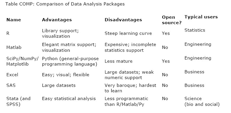
from:
http://assets.doloreslabs.com/blog/oconnor_biewald_beautiful_data_final_nonlayout_20090803_20090327.pdf
SPSS is a
bit harder than Excel but gives you a much wider menu of statistical
analysis. You don't have to write
computer programs like some of the others – you can just use drop-down menus
and point and click.
You might be
tempted to just use Excel; resist! Excel
doesn't do many of the more complex statistical analyses that we'll be learning
later in the course. Make the investment
to learn a better program; it has a very good cost/benefit ratio.
1. The
Absolute Beginning
Start up
SPSS. On any of the computers in the
Economics lab (6/150) double-click on the "SPSS" logo to start up the
program. In other computer labs you
might have to do a bit more hunting to find SPSS (if there's no link on the
desktop, then click the "Start" button in the lower left-hand corner,
and look at the list of "Programs" to find SPSS).
Sometimes
double-clicking on a file that is associated with SPSS doesn't work! Same if you
try to download a file and automatically start up SPSS. So start SPSS from the Start bar or desktop
icon.
SPSS usually
brings up a screen like the one below asking "What would you like to do?" which offers some
shortcuts. Just "Cancel" this
screen if it appears (later, as you get more familiar with the program, you
might find those shortcuts more useful).

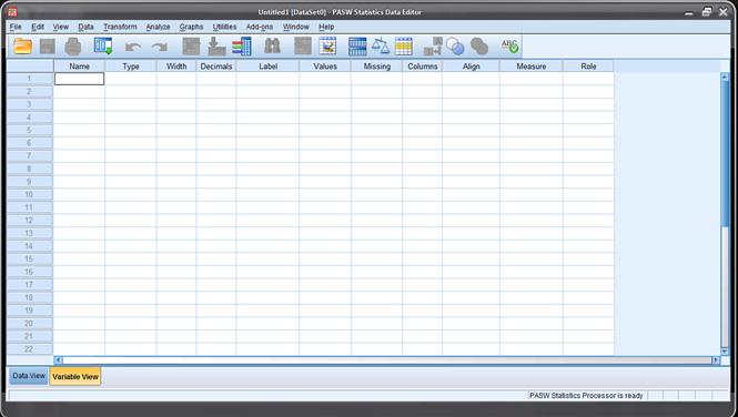
2. Load
a SPSS Dataset
When SPSS
starts, you will be in the "SPSS
Data Editor" which
looks like this.
![]()
Click on
"File" then choose "Open" then "Data…" [not "File/Open Database"
– that's different].
To open the
ATUS data, download it from the class webpage onto your computer desktop. Start SPSS.
Then "File \ Open \
Data..." and find
"ATUS_2003-09.sav".
SPSS has two tabs (at the bottom left, in the yellow circle above) to change the way you view your data. The "Data View" tab shows the data the way it would look if it were on an Excel sheet. The "Variable View" tab shows more information on the particular variable – most importantly, the "name", "label", and "values". The Name is how SPSS refers to the variable in its menus – these names tend to be inscrutable but you can think of them as nicknames. The Label gives more details, so use the mouse to expand that column so that you can read more. Then values tells you useful information about how the variable is coded.
3. Save
your Work!
After you've
made changes, you don't want to lose them and have to re-do them. So save your dataset! ("File" then "Save")
You might want to give it a new name
each time, so that you can easily revert back to an old version if you really
screw up on some day.
The
computers in the lab wipe the memory clean when you log off so back up your
data. Either online (email it to
yourself or upload to Blackboard) or use a USB drive. Also, figure out how to "zip" your
files (right-click on the data file) to save yourself some hours of up/download
time…
4. Getting
Basic Statistics
From either
the "Data View" or "Variable View" tab, click "Analyze" then "Descriptive
Statistics" then
"Descriptives":

This will
bring up a dialog box asking you which variables you want to get Descriptive
Statistics on.

Click on the
variable you want. Then click the arrow
button in the center box, which will move the variables into the column labeled
"Variable(s)". If you make a mistake and move the wrong
variable, just highlight it in the "Variable(s)" column and use the arrow to
move it back to the left.
Then click
"OK" and let the computer work.
If you want
a bunch that are all together in the list, click on the first variable that you
want, then hold down the "Shift" key and click on the last variable -- this
highlights them all. If you want a bunch
that are separated, hold down the "Ctrl" key and click on the ones you
want.
Later, once
you're feeling confident, click on "Options" to see what's there.
5. Create
New Variables, like Age-squared or Interaction Age*Dummy, or take logs or
whatever
We often
create new variables. One common
transformation is taking the log. This
is a common procedure to cut down the noise and help to examine growth
trends. Click on "Transform" and then
"Compute…". This will bring up a dialog box labeled
"Compute Variable".
Type in the
new variable name (whatever you want, just remember it!) under "Target Variable". (You can click 'Type & Label"
if you want to enter more info that can remind yourself later.) For example we'll find the log (natural log)
of weekly earnings.

Under "Target Variable" type in the new name, "ln_earn" or whatever and then in "Numeric Expression" you tell it what this new variable is. You can make any complicated or convoluted
functions that are necessary for particular analyses; for now find the "Function Group"
to click on "Arithmetic" and then in the "Functions and Special Variables" list below find "Ln". Double-click it and see that SPSS puts it up
into the "Numeric Expression" box with a (?)
in the argument. Double-click on the
variable, weekly earnings (TRERNWA), that you want to use and then hit
"OK".
You'll get a
bunch of errors where the program complains about trying to find the log of
zero, but it still does what you need. For
wages, where many people have wage=0, we often use lnwage
= ln(wage + 1) which eliminates the problem of ln(0) that returns an error; for most other people the
distinction between ln(1000) and ln(1001)
is tiny. You can go back and re-do your
variable if you're feeling a need to be tidy.
We often
need to recode using logical (Boolean) algebra, so for example to make a
variable "Hispanic" you'd type "Hispanic"
into the Target Variable, then click the "( )"
button (see the yellow circle in the screenshot below) to get a parenthesis,
double-click the variable that codes ethnicity so as to get PEHSPNON
in the "Numeric Expression" and then add "=1"
to finish, so getting a relationship that Hispanic is defined as: (PEHSPNON = 1). SPSS
understands that whenever that relation is true, it will put in a 1; where
false it will put in a 0.


There are
other logical buttons (also in the yellow circle above) for putting together
various logical statements. Now that the
Census asks people for detailed race info (could be African-American only or
Asian or bi-racial or tri-racial in various combinations – see the online note
on ATUS for more details), researchers might aggregate together everyone who
replies that they are all or part African-American. So maybe create AfricanAmerican
as (PTDTRACE = 2) | (PTDTRACE =
6) |(PTDTRACE = 10) |(PTDTRACE = 11) |(PTDTRACE = 12) |(PTDTRACE = 15) |(PTDTRACE
= 16) |(PTDTRACE = 19) . (The line up and down, |,
represents the logical "OR"; the tilde, ~,
is logical "NOT".)
If you
wanted to create a variable for those who report themselves as African-American
and Hispanic, you'd create the expression (AfricanAmerican = 1) & (PEHSPNON = 1), etc.
If we want more combinations of variables then we create those. Usually a statistical analysis spends a lot of time doing this sort of housekeeping – dull but necessary.
6. Re-Coding
complicated variables (like race, education, etc) from inital
data
Often we
have more complicated variables so we need to be careful in considering the
"Values" labels. For instance in the ATUS, as you look at the
"Variable View" of your dataset, one of the
first variables in the dataset has the name "PEEDUCA",
which is short for "PErson EDUCation
Achieved" – the person's education level.
But the coding is strange: under "Values"
you should see a box with "…" in it – click on that to see
the whole list of values and what they mean.
You'll see that a "39" means that the person
graduated high school; a "43" means that they have a
Bachelor's degree. Without that "Values"
information you'd have no way to know that.
It also means that you must do a bit of work re-coding variables before
you work with the data. The variable
"TEAGE" (which is the person's age)
has numbers like 35, 48, 19 – just what you'd expect. These values have a natural interpretation;
you don't need a codebook for this one! The
variable "TESEX" tells whether the person is
male or female – but it doesn't use text, it just lists either the number 1 or
2. We could guess that one of those is
male and the other female, but we'd have to go back to "Variable View" to look at "Values"
for "TESEX" to find that a 1 indicates a
male and a 2 indicates female.
Start with
"TESEX" to create, instead, a dummy
variable (that takes a value of just zero or one) called "female"
that is equal to one if the person is female and zero if not. To do this, click "Transform" then "Compute…" which will bring up a dialog
box. The "Target Variable" is the new variable you are creating; for this
case, type in "female". The "Numeric Expression"
allows considerable freedom in transforming variables. For this case, we will only need a logical
expression: "TESEX = 2". You can either type in the variable name,
"TESEX", or find the variable name in
the list on the left of the dialog box and click the arrow to insert the
name.
Later you
might encounter cases where you want more complicated dummy variables and want
to use logical relations "and" "or" "not" (the
symbols "&", "|",
"~") or the ">="
or multiplication or division. But in
this case, we just need "TESEX
= 2" which SPSS
interprets as telling it to set a value of 1 in each case where that logical
expression is true, and a value of zero in each case where that expression is
false. If you go to "Data View" and scroll over (new variables are all the way on
the right) you can check that it looks right.
Next we'll
create the racial variables. We'll
create dummy variables for "white", "African-American",
"American Indian/Inuit/Hawaiian/Pacific Islander", and
"Asian." We'll lump together
the people who give multiple identities with those who give a single one (this
is standard in much empirical work, although it is evolving rapidly).
So "Tranform/Compute…" and label "Target Variable" as "white" with "Numeric
Expression" "PTDTRACE=1". Then "afam" is "( PTDTRACE=2)
| (PTDTRACE=6) | (PTDTRACE=10) | (PTDTRACE=11) | (PTDTRACE=12) | (PTDTRACE=15)
| (PTDTRACE=16) | (PTDTRACE=19)"
– note the parentheses and the "or" symbol. "Asian" is "( PTDTRACE=4) | (PTDTRACE=8)". "Amindian" is "( PTDTRACE=3)
| (PTDTRACE=5) | (PTDTRACE=7) | (PTDTRACE=9) | (PTDTRACE=13) | (PTDTRACE=14) |
(PTDTRACE=17) | (PTDTRACE=18) | (PTDTRACE=20) | (PTDTRACE=21)". (Many of these codings
of multiple races could be argued – you can make changes if you wish.)

Next we
create a dummy variable for "Hispanic". Again use "Transform/Compute…" and label "Target
Variable" as "Hispanic" with "Numeric
Expression" of
"(PEHSPNON = 1)".
Next create
dummy variables for education: a dummy for no high school "ed_nohs", for high school but no
further "ed_hs", for some college "ed_scol", for a bachelor's degree
"ed_coll", and for more than a 4-year
degree "ed_adv". "Transform/Compute…", set "Target
Variable" as "ed_nohs" and "Numeric
Expression" as
" PEEDUCA <39". Then "ed_hs" is " PEEDUCA =39"; "ed_scol" is "( PEEDUCA >39)&( PEEDUCA <43)"; "ed_coll" is " PEEDUCA =43"; "ed_adv" is " PEEDUCA >43".
Then run
"Descriptive Statistics" to make sure everything looks right – your
dummy variables should have min=0 and max=1, for example!
7. Data
Sub-Sets
Often we
want to compare groups of people within the dataset to each other, for example
looking at whether men or women spend more time with their family or watching
TV or whatever. Comparisons are often
more useful than just raw numbers because comparisons allow us to begin to
judge which differences are substantial.
Do this with
"Data" then "Select Cases..." to get a screen like this:

Usually we
select cases "If condition
is satisfied" so
choose that, then click on "If..."
This brings
up a dialog box that looks like the "Compute Variable" box from
above. If we have already created a
dummy variable that has values of only zeroes and ones then you can just put
that into the "Select Cases" box.
If you want a more complicated set then you can build it up using the
logical notation that we discussed above.
So suppose you want to look at just the subgroup of women between the
ages of 18-35. Then we would enter
"(TESEX = 2) & (TEAGE
> 18) & (TEAGE <= 35)". Click "Continue". Make sure the output is "Filter out
unselected cases" (you don't usually want to permanently delete the
unselected cases!). Then all of your
subsequent analyses will be done for just that subgroup.
Often an
analysis will be more concerned with whether a particular item is done rather
than how long – for example, when looking at working, whether a person has a
second job (so time spent working second job is greater than zero) is probably
more important than just how long they spent working at this second job. So often the "if..."
statement will be of the form, "X
> 0" for whatever
variable, X, you're considering.
Later on, we
will learn some more sophisticated ways of doing it but for now this is
straightforward and clear. It will allow
you to do the homework assignment.
8. Example
I will do an
example to make this a bit clearer. We
will look at the difference in how much time male and female college students
spend watching TV. (I hope that for you
the answer is "zero"!)
Open the
ATUS 2003-2009 dataset.
First use
"Transform \ Compute ..." to create a new variable, tv_time, which we set equal to the sum of T120303, watching
non-religious TV, and T120304, watching religious TV. (Should we include T120308, playing computer
games?)
Use "Transform
\ Compute ..." to
create another variable, educ_time, which is the sum
of time spent doing things relevant to education, T060101 + T060102 + T060103 +
T060104 + T060199 + T060301 + T060302 + T060303 + T060399. (Time spent in class and time spent doing
homework, mainly.)
I'll also
create "ratio_TV_study" that is the ratio
of TV_time to educ_time.
Run "Analyze \ Descriptive Statistics \ Descriptives ..."
to check that these seem sensible:
|
Descriptive
Statistics |
|||||
|
|
N |
Minimum |
Maximum |
Mean |
Std.
Deviation |
|
tv_time |
98778 |
.00 |
1417.00 |
165.2058 |
168.33963 |
|
educ_time |
98778 |
.00 |
1090.00 |
16.3008 |
79.47292 |
|
ratio_TV_study |
5974 |
.00 |
120.00 |
1.0450 |
3.00829 |
|
Valid N (listwise) |
5974 |
|
|
|
|
Note that
the average for "educ_time" is low because
most non-students will report zero time spent studying. All of those zero values returned errors when
computing the ratio, so this has only 5974 reports of people with more than
zero time studying.
Use
"Data \ Select Cases ... " to select only college students (those for
whom the 13th variable, TESCHLVL, is equal to 2).
Now to
compare men and women I will use "Data
\ Split File ... "
to split into two groups and compare them – the program will do this
automatically for all subsequent analysis.
This Split
File screen is:
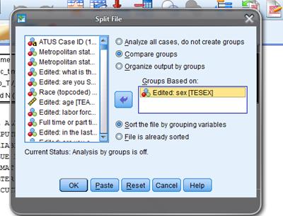
Now when I
run the same "Descriptives" as before, this
time I get the output subdivided:
|
Descriptive
Statistics |
||||||
|
Edited: sex |
N |
Minimum |
Maximum |
Mean |
Std.
Deviation |
|
|
= "Male" |
tv_time |
2018 |
.00 |
860.00 |
127.1665 |
138.93259 |
|
educ_time |
2018 |
.00 |
1051.00 |
112.6056 |
186.01012 |
|
|
ratio_TV_study |
784 |
.00 |
75.00 |
.8390 |
3.02939 |
|
|
Valid N (listwise) |
784 |
|
|
|
|
|
|
=
"Female" |
tv_time |
3581 |
.00 |
1100.00 |
111.4739 |
124.86338 |
|
educ_time |
3581 |
.00 |
1090.00 |
104.8176 |
173.84758 |
|
|
ratio_TV_study |
1450 |
.00 |
120.00 |
.9117 |
4.04470 |
|
|
Valid N (listwise) |
1450 |
|
|
|
|
|
This shows
that male college students watch an average of 127 minutes of TV per day and
devote an average of 113 minutes to school; females watch 111 minutes of TV and
devote 105 minutes to their studies. Men
watch more TV but also spend a bit more time on school so the average ratio of
time spent watching TV to time spent on school is .91 for women and .84 for
men.
Finally I'll
show a graph,
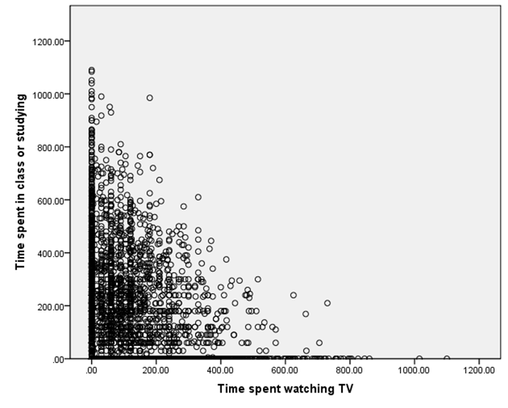
Note that
there are quite a number of respondents who spent zero time studying or zero
time watching TV. We would expect a
downward relation since it is like a budget set: the more time is spent
watching TV, the less is available to do anything else.
To get this
graph, choose "Graphs \
Chart Builder ..."
and drag the elements to where you want them, like this,
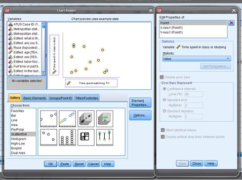
This is the
first type of "Scatter/Dot" graph.
For this
graph I removed the split, since it didn't look like there were significant
differences between men and women in that regard – the same "Data \ Split File ... " but now "Analyze all
cases."
I can create
a histogram of the ratio of time spent watching TV to time spent studying, 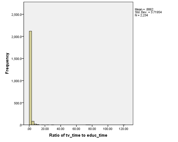
But this
isn't much use since it's dominated by the few extreme values of people who
spent 100 or more times as many minutes in TV as studying. So this histogram,
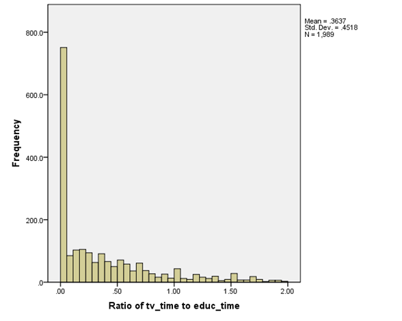
plots only
those with a ratio less than 2.
(To make
this chart, I used "Graphs
\ Chart Builder ..."
and then chose "Bar." When you
put in just one variable on the x-axis it assumes you want a Histogram.)
Now you can
go on to do your own analysis, maybe by race/ethnicity? Or go back and add in video game
playing? Of the people who didn't watch
TV, were there a larger fraction of men or women?
Some Shortcuts
You can use "Analyze \ Descriptive Statistics \ Explore..." which asks you to put in the
"Dependent List" which are the variables, whose
means you want to find, and then the "Factor List"
which defines categories, by which the subgroup means are found. So, for example, if you wanted to look at the
time sleeping, depending on whether there are kids in the house, you could put
"Time Sleeping" into the "Dependent List" and then "Presence of Household Children" into the "Factor List".
You can get fancier if you create your own
factors – suppose you wanted to look at time sleeping for African-American,
Hispanic, Asian, and whites at 5 levels of education each (without highschool diploma, with just diploma, with some college,
with 4-year degree, with advanced degree) – for a total of 4 x 5 = 20 different
categories. So create a new variable
that takes the values 1 through 20 and carefully code it up for each of those
categories. Then put that into
"Factor" in "Explore" and let the machine do your work.
SPSS also
has "Analyze \ Compare Means" but we won't get to that yet (although
you're welcome to explore it on your own!).