|
Lecture Notes 3 Supplement Production Economics of the
Environment and Natural Resources/Economics of Sustainability K Foster, CCNY, Spring 2011 |
|
|
Production
Externalities
In the simplest case, we can examine a firm making a single private (rival and excludable) output and incidentally a single public (nonrival and nonexcludable) output (for now, we assume that this public good is disliked). An easy example could be a power plant which makes electricity and pollution. (Actually a variety of sorts of pollution, which affect different groups of people: carbon, mercury, NOX, and sulphur dioxide are the main ones.)
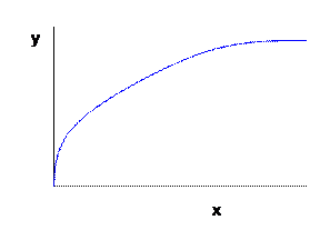
In this case the production can be shown as being like a production possibility frontier but with the pollution increasing along with the output, something like:
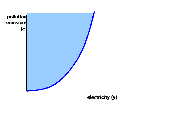
The firm can choose any combination of electicity & pollution within the light blue area. Clearly, however, the firm would be foolish to choose a point inside the area; the points at the dark blue line are efficient. These are the production possibility frontier. They are efficient because there is no way to increase the output of electricity without also increasing the output of pollution (this would not be true for points in the interior).
|
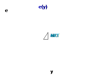
At any point along the
frontier of production possibilities, we can define the marginal rate of
transformation as the change in output of pollution per change in output of
electricity – the slope of the line.
With the notation of e for pollution emissions and y for the output of
the firm, the marginal rate of transformation, MRT, here is |
|

This interpretation of the choice along the production possibility frontier as representing a choice of marginal rate of transformation allows us to compare firms and make statements about the relative efficiency.
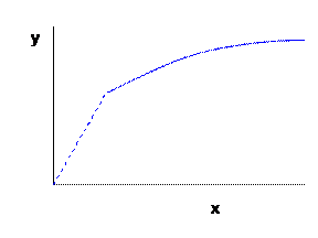
Suppose there are two firms which, for some reason or another, have different emissions per unit of output. Graphically this would be represented as:
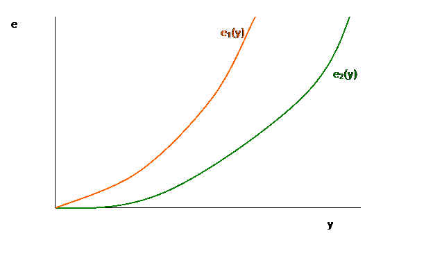
If they each produced the same amount of emissions, they would of course be able to generate different output levels, but their marginal rates of transformation would also be different.
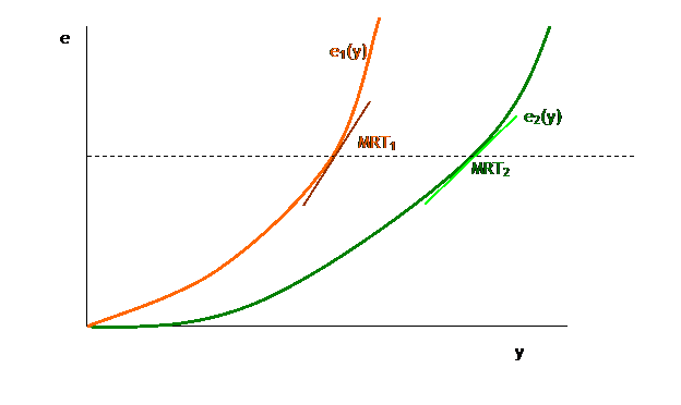
Clearly the marginal rate of transformation of firm 2 is lower than the marginal rate of transformation of firm 1. This means that when firm 2 generates one more unit of output, it creates fewer emissions than firm 1 does. This means that, if firm 2 were to make one more unit of output while firm 1 made one unit less – keeping the total output of the two firms at the same level, the increase in emissions from the second firm would be (in absolute value) less than the decrease in emissions from the first firm. So total emissions would be smaller even though the output was kept constant.
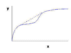
Consider a simple numerical example, where ![]() but
but ![]() . This is
plotted as:
. This is
plotted as:
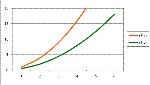
If emissions of each firm are 16, then firm 1 is producing 4 units of electricity while firm 2 is producing 5.66 units of electricity. If firm 2 produced one more unit of electricity its emissions would rise to 22.16, an increase of 6.16. If firm 1 produced one less unit of electricity its emissions would fall to 9, a decrease of 7. So if, instead of both firms producing 16 units of emissions, firm 1 produced less and firm 2 produced more, the overall production of electricity could remain constant while emissions fall.
We can continue this trade-off as long as the marginal rates of transformation are unequal. It is only when the marginal rates of transformation are equal that there will be a total efficient way of getting the most output with the least amount of harmful emissions.
With a bit more math, we can find the point where the MRTs for each firm will be equal.
|
Multiple Inputs |
|
|
It is rarely quite appropriate to consider an output to be perfectly free, since there are usually at least technological considerations. So we can return to our usual marginal conditions, modified for the firm. Consider a firm which has multiple inputs available for making the output, each of which is useful and productive. Each input has a cost (or wage, if we extrapolate from the case of hiring workers) denoted wi.
We typically assume that, holding all of the other inputs constant, increases to just one input will have a steadily-decreasing effect on increasing output. Graphically, this says that for each input, xi, i=1, 2, … N, output, y, increases as:
So, just as with the consumer's diminishing marginal
utility, the firm faces diminishing marginal productivity. Just as with the consumer, we define the
production function as ![]() and the
marginal product of each input as the partial derivative,
and the
marginal product of each input as the partial derivative, ![]() .
.
Also as noted previously, the fact that each individual marginal product is diminishing does not mean that production overall has diminishing returns to scale – where 'scale' refers to a case where all of the relevant inputs are increased. As a simple example, most offices generally operate with each employee getting a computer. Buying more computers without hiring more people might increase output, but at a diminishing rate; the same would hold true for hiring more people without getting more computers. But getting more of both could allow the business to expand.
The firm will maximize profits by choosing inputs such that
(in the long run), the ratios of ![]() , marginal productivity per cost of each input, is
equal. The explanation should, by now,
be typical: if spending $1 more on input i increased output by more than
spending $1 more on input j, then the firm should decrease spending on input i
while increasing spending on input j.
This will not only allow the firm to make more output more cheaply but
also tend to bring down the marginal productivity of input j while increasing
the marginal productivity of input i, so that in equilibrium we have
, marginal productivity per cost of each input, is
equal. The explanation should, by now,
be typical: if spending $1 more on input i increased output by more than
spending $1 more on input j, then the firm should decrease spending on input i
while increasing spending on input j.
This will not only allow the firm to make more output more cheaply but
also tend to bring down the marginal productivity of input j while increasing
the marginal productivity of input i, so that in equilibrium we have ![]() .
.
If one input has a price which is increased (say, by some environmental regulation) then this input will be used less. This is the substitution effect (see from marginal condition).
There is also a Scale Effect. As the cost of production rises, the quantity of output demanded will fall, so fewer of all types of input will be demanded.
Also, if that input is non-excludable like polluted air or water, then other industries could see their costs fall, so input used more – a different substitution effect. Also a different scale effect.
Hicks-Marshall rules
of Derived Demand
Pass-through of price changes depends on Hicks-Marshall rules of Derived Demand:
a. Demand for input is more elastic when
i. technical substitution is easy
ii. input is supplied elastically
iii. input cost share is high
iv. demand for output is elastic
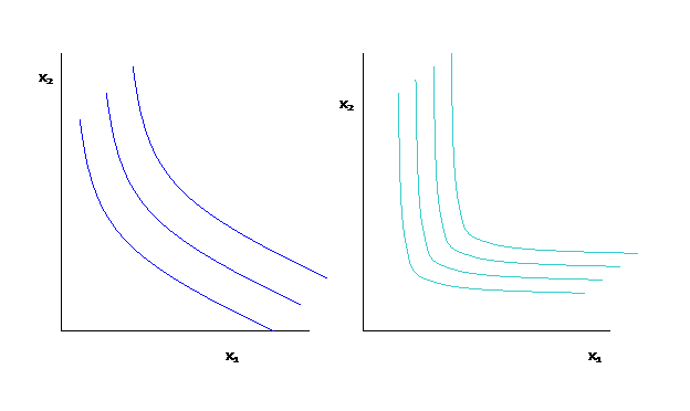
Take each one in turn. #1 means that isoquants are as on left not on the right,
#3, that cost share is high, means that there is a substantial pass-through of this particular input cost,
#2, that input is supplied elastically, means that if #1 is fulfilled (it is technologically feasible to get more or less of the input), it will not change the price of that input to buy more or less,
#4, that demand for the output is elastic means that changes in price have a significant change in demand for the output.
Firms in Perfect
Competition
Assume that firms want to maximize profit, p, which is Revenue minus Cost. This is far from a perfect description of the world of course.
The first question – to make a particular quantity of output, what is the cheapest way to make it? – gives us the single essential number: the cost of that amount of output. The cost of this output is the only important item that the firm, when choosing amount of output to produce, needs to know. It does not need to know the quantities of inputs or relative costs. This split can also be thought of as reflecting a firm's organization: there is the corporate level that makes the decisions about how much product to make, if those output levels have a particular cost. Then these decisions are communicated to the plants that make the output, where each plant manager is told to make a particular amount of output, using the cheapest input mix possible. The plant manager doesn't need to know how a particular quantity of output was chosen; the corporate level doesn't need to know details of how that output is made, just the cost.
At this level we are not paying attention to questions of corporate structure. Given the decision structure from above, we might think of the plant managers as being a separate firm, outsourcing production. (A brand-name computer maker buys chips from a separate company; it doesn't need to know details of how the chips are made, indeed that might be a close-held secret. All it needs to know is the cost.) Our modern economy has many such firms providing corporate services, from high-level research down to the company cafeteria.
We begin our analysis at the base, at the level of the plant, which is given an order for a particular quantity of output and must choose how to most cheaply make it. Again we divide the decision into two parts: first asking what is physically possible (what inputs can make the output) and then asking which combination is cheapest.
This plant is described as having a production function
where inputs ![]() are transformed
into outputs by way of a production function:
are transformed
into outputs by way of a production function: ![]() . We could
imagine a wide variety of production functions but we assume that it has some
basic properties. Note that, where, in
the consumer problem, we were reluctant to make restrictions directly to the
utility function and instead discussed assumptions about the underlying
preferences, that was because utility was un-measurable and only a convenient
descriptive device. Production is more
easily measured as long as there is some physical output: tons of steel or
pairs of sneakers or casks of beer. So
we make assumptions directly about the production function.
. We could
imagine a wide variety of production functions but we assume that it has some
basic properties. Note that, where, in
the consumer problem, we were reluctant to make restrictions directly to the
utility function and instead discussed assumptions about the underlying
preferences, that was because utility was un-measurable and only a convenient
descriptive device. Production is more
easily measured as long as there is some physical output: tons of steel or
pairs of sneakers or casks of beer. So
we make assumptions directly about the production function.
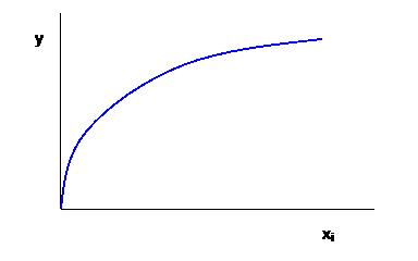
We typically assume that the production function is increasing (so more inputs lead to more output), continuous, and convex (or something like convex).
One Input
The simplest case is where one input makes one output, so we
simply have ![]() . The marginal
product of the input is how much additional output is made by adding more
input, or
. The marginal
product of the input is how much additional output is made by adding more
input, or ![]() , which is the slope of the graph.
, which is the slope of the graph.
The assumption of ![]() being an
increasing function (i.e. that
being an
increasing function (i.e. that ![]() ) is anodyne.
Just as with utility, if output actually falls when inputs rise then you
don't need an advanced degree to figure out that you should cut back. The interesting problem occurs when output
could still be increased and you want to figure out if it is profitable.
) is anodyne.
Just as with utility, if output actually falls when inputs rise then you
don't need an advanced degree to figure out that you should cut back. The interesting problem occurs when output
could still be increased and you want to figure out if it is profitable.
The assumptions of continuity and convexity don't seem as obvious. But they can be solved if we think of the firm's problem over a slightly longer period. Suppose that a firm's underlying physical process of production is discontinuous: it takes at least 100 units of input in a day to make 100 output units, but less than 100 of the input just won't even start up the machine. Is the firm's production function to be considered discontinuous? Well what if the firm got orders for 50 units of output per day – what would it do? Clearly it could just run the machine every other day, and average 50 units of output with 50 units of input per day. If orders run at 80 per day then the machine is run on 4 out of 5 days, and so forth. Of course this assumes that the output is storable and that the time over which we are speaking is relatively short (more on this later).
The convexity assumption comes by the same assumption. If the firm can make 100 output with 100 input then it could make at least half as much output with half the input. (On the graph, any chord drawn between 2 points will lie on or beneath the production function.) If there were non-convexities in the underlying physical process then, again, production could be structured to avoid these.
The convexity assumption is also why we often talk about a
"Law" of Diminishing Marginal Product. It is reasonable to assume that the Marginal
Product, ![]() , is diminishing (or at least not increasing) because
if it were increasing then, as in the graph above, the firm would want to
figure out ways to exploit this.
, is diminishing (or at least not increasing) because
if it were increasing then, as in the graph above, the firm would want to
figure out ways to exploit this.
More Than One Input
But clearly assuming just one input to the production function is restrictive. I can't think of too many things that are produced in that way (except for the world's oldest profession). We want to consider multiple inputs.
We limit ourselves to two inputs because that allows easy
graphing and still gets to most of the complexities. But you should be able to see how the number
of inputs could be increased. Now assume
that the production function is given as ![]() . Again we
assume that the production function is increasing, continuous, and convex. Now define each input's Marginal Product:
. Again we
assume that the production function is increasing, continuous, and convex. Now define each input's Marginal Product: ![]() , where we use the function notation to remind
ourselves that the MP for each input is likely to be different, for different
levels of each input. This is important
– there are likely to be complementarities in production. The Marginal Product of one input is likely
to depend on the levels of other inputs as well. (For example we often hear statistics that
workers in third-world countries are not as productive as
, where we use the function notation to remind
ourselves that the MP for each input is likely to be different, for different
levels of each input. This is important
– there are likely to be complementarities in production. The Marginal Product of one input is likely
to depend on the levels of other inputs as well. (For example we often hear statistics that
workers in third-world countries are not as productive as
Again we assume diminishing marginal products, that ![]() falls as input
1 rises (holding constant input 2) and vice versa. This "holding constant" part is
particularly important since, while in the long run we might be able to
increase output by increasing both inputs, in the short run one input or the
other is usually less flexible. Consider
the typical office worker nowadays, who usually gets one computer. If a company hires more people without buying
more computers, then the productivity of the new people (whatever their
talent!) will be limited as they have to jostle for computer time. Similarly if the company got new computers
without hiring new people – a few people might get multiple computers on their
desks, and some might be more productive with those new computers, but not very
much.
falls as input
1 rises (holding constant input 2) and vice versa. This "holding constant" part is
particularly important since, while in the long run we might be able to
increase output by increasing both inputs, in the short run one input or the
other is usually less flexible. Consider
the typical office worker nowadays, who usually gets one computer. If a company hires more people without buying
more computers, then the productivity of the new people (whatever their
talent!) will be limited as they have to jostle for computer time. Similarly if the company got new computers
without hiring new people – a few people might get multiple computers on their
desks, and some might be more productive with those new computers, but not very
much.
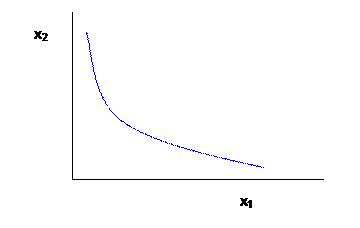
We graph the interaction of two inputs to make a particular amount of output by showing an "isoquant" – a very unlovely word! An isoquant connects together different amounts of inputs that give the same level of output. (Analogous to indifference curves.)
In a simple case, say we want to move a specified amount of dirt (dig a hole or fill in a hole or whatever). We could do it with a lot of people with basic tools, or gradually give some people more powerful tools and hire fewer people, all the way to having only one or two people running gigantic machines. There's no necessary reason that one or the other is better, the firm only cares about prices. If people can be hired cheaply then the firm will use more people; if machines are cheap then the firm will use machines.
We could imagine perfect complements or perfect substitutes in production or anything between. Typically the isoquants are assumed to be convex, for reasons similar to what was explained above in the one-input case.
As you can probably guess, we want to find an equation for
the slope of the isoquant, which is called the Technical Rate of Substitution,
or TRS. The TRS tells us how many of
input 2 must be added, when one unit of input 1 is removed, to keep output
constant. Again to figure out the TRS,
imagine that we cut input 1 by ![]() units – how
much would output be expected to fall?
We would expect
units – how
much would output be expected to fall?
We would expect ![]() . But if we
wanted to keep
. But if we
wanted to keep ![]() constant then we would need to balance this with an
infusion of input 2, in amount of
constant then we would need to balance this with an
infusion of input 2, in amount of ![]() , just enough that
, just enough that ![]() . From this we
see that
. From this we
see that ![]() .
.
Just as with the indifference curves, we expect that there
should be a diminishing TRS as input 1 is increased. This comes about from the assumption that
each input has diminishing marginal productivity: as input 1 increases and
input 2 is cut, ![]() will fall and
will fall and ![]() will rise so
TRS will fall as input 2 rises.
will rise so
TRS will fall as input 2 rises.
Short Run vs Long Run
Often one input is more flexible than the other. This means that our analysis should distinguish between the short run (when one input is fixed) and the long run (when both inputs are flexible). Often we assume that labor is flexible and capital (the machines) are fixed since building, say, a new assembly line takes time. But other firms might have different rankings – universities have tenured faculty, many of whom have been there longer than some of the buildings on campus!
In the long run we want to consider the possibility of
returns to scale. If a firm doubled its
inputs, what would happen to outputs? If
output doubled exactly then a firm would have constant returns to scale
(CRS). If output increased by more than
double then the firm has increasing returns to scale (IRS). If output increased by less than double then
there are decreasing returns to scale (DRS).
To put this a bit more abstractly, we compare the output from doubling
the inputs, ![]() , with twice the original output,
, with twice the original output, ![]() . If
. If ![]() then production
is CRS; if
then production
is CRS; if ![]() then IRS; if
then IRS; if ![]() then DRS. Or, more generally, for any scale factor
then DRS. Or, more generally, for any scale factor ![]() , if
, if ![]() then production
is CRS; if
then production
is CRS; if ![]() then IRS; if
then IRS; if ![]() then DRS.
then DRS.
Profit Maximization
A firm's profits are revenues minus costs, so a firm selling
n different output goods, each for
price pi, and using m different inputs, each with cost wj, would have profit ![]() .
.
First note that the costs must all be put into the same units – dollars per time unit. Which raises the question, if a firm buys, say, a truck that is expected to last for 5 years, how is this cost compared against the daily wage of the person driving it? To answer this we suppose that another company were set up that just rented out trucks: it goes to the bank, gets a loan to buy the truck, and then charges enough per day to pay off the loan per day. We consider that, even if a company doesn't actually rent the truck but actually buys it, that it could have rented the truck. So the rental rate is the correct cost of that capital good. Again, in the real world more and more companies are separating their daily operations from their loan portfolio and renting equipment. If you work at an office, you know that most photocopiers are rented. Airlines rarely own their own jets, they rent them. Offices are usually rented space.
The companies have figured out that correctly measuring costs allows them to make better decisions. Capital goods which are owned and given away internally as if they had zero cost are not efficiently used.
Economists also measure costs differently from the way that accountants do regarding payments to shareholders/owners. If a public company has an IPO and sells its shares for $100 each, then those shareholders expect something in return. They expect that the dividends (and/or capital gains) will return them as much money as if they had invested their $100 in some other venture. So the company had better return $8 per year if the investors could have gotten 8% returns. An accountant would count this $8 per share as a "profit" but economists see that as a cost to be paid to shareholders for the use of their money (their capital). If the firm were to return just $6 then the shareholders would be angry and the firm would be in trouble; if the firm returns $12 then the shareholders are delighted.
So economists often talk about "zero profits" being a general case, which makes people wonder how much economists know about the real world since any business newspaper daily reports companies making "profits". But we're just counting different things. If the regular return to capital is 8% then, if the firm makes $8 that the accountants call profit, we call it a cost and report that the firm made zero economic profit.
Profit Maximization
with One Input
This means
![]() subject to
subject to ![]() . Hiring one
more unit of input will raise the firm’s cost by
. Hiring one
more unit of input will raise the firm’s cost by![]() ; this one additional unit of input will raise output
by
; this one additional unit of input will raise output
by ![]() and so revenues
will rise (assuming no market power) by
and so revenues
will rise (assuming no market power) by ![]() , which is the value of the marginal product. If
, which is the value of the marginal product. If ![]() then the firm
should hire more inputs; if
then the firm
should hire more inputs; if ![]() then the firm
should hire fewer inputs; so in equilibrium
then the firm
should hire fewer inputs; so in equilibrium ![]() .
.
Note that, if one input is fixed, then even the two-input model becomes, in the short run, just this problem of profit maximization with one input.
Profit Maximization
with Multiple Inputs
Now the firm is to ![]() subject to
subject to ![]() . Again the
same logic applies. Hiring one more unit
of input one will raise the firm’s costs by
. Again the
same logic applies. Hiring one more unit
of input one will raise the firm’s costs by ![]() and raise
revenues by
and raise
revenues by ![]() so in
equilibrium
so in
equilibrium ![]() and
and ![]() . Also these
imply that our usual bang-for-the-buck marginal conditions apply, that
. Also these
imply that our usual bang-for-the-buck marginal conditions apply, that ![]() which is the
tangent condition that the slope of the isocost equals the slope of the
isoquant at optimum. This condition
gives the long-run profit maximizing combination of inputs to be used, which
allows us to derive the long-run cost function.
which is the
tangent condition that the slope of the isocost equals the slope of the
isoquant at optimum. This condition
gives the long-run profit maximizing combination of inputs to be used, which
allows us to derive the long-run cost function.
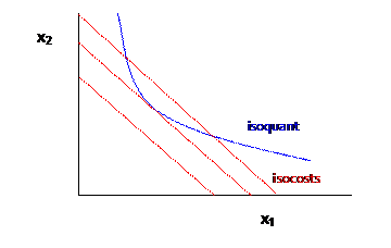
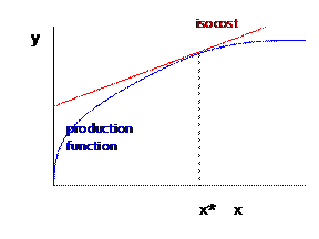
To make a particular amount of output, in the long run the firm minimizes cost by choosing to produce with the inputs set at the tangency.
Cost
Minimization/Profit Maximization
The firm’s problem to maximize profits generates a dual (sometimes easier) problem, which is how to minimize costs subject to a constraint of making a particular amount of output. If the firm wanted to minimize costs without that constraint, clearly setting y=0 would be best.
If the firm wanted only to maximize revenue (or if the input
were costless) then the firm would ![]() subject to
subject to ![]() . To figure
this out, we just need one definition: Marginal Revenue.
. To figure
this out, we just need one definition: Marginal Revenue.
Marginal Revenue
Marginal Revenue, MR, is the change in revenue per change in
output, ![]() . If price is a
function of the level of output (e.g. the firm has monopoly power) then MR can
be a complex function. However for now
we will start simple and assume that the firm operates in a competitive market
so the price is outside its control. In
this case, the increase in revenue from selling one more unit of output is the
price, p.
. If price is a
function of the level of output (e.g. the firm has monopoly power) then MR can
be a complex function. However for now
we will start simple and assume that the firm operates in a competitive market
so the price is outside its control. In
this case, the increase in revenue from selling one more unit of output is the
price, p.
A firm that wanted just to maximize revenue would expand production as long as MR>0 and only stop when MR=0, when producing more output would no longer raise its Revenue.
Most firms, however, do not simply care about maximizing revenue; they want to maximize profits. (Particular parts of firms, however, might want to maximize revenue: for instance, most sales people are paid commissions on the sales they generate not necessarily the profits.)
A firm that wants to maximize profits will also have to take account of Marginal Cost. It is also convenient to figure other cost definitions.