|
Lecture Notes 4 Economics of the
Environment and Natural Resources/Economics of Sustainability K Foster, CCNY, Spring 2011 |
|
|
|
Intertemporal Choice and Discount Rates |
|
|
In general people value a sum of money paid in the future less than a sum of money paid now. This is represented by a "discount" factor: $100 in the future is worth $100*D now, where D<1.
The reason for this goes back to one of the most basic propositions of economics, opportunity cost. A thing's value is its opportunity cost, what must be sacrificed in order to get it. The opportunity cost of $100 in one year is not $100 now – I could put less than $100 in the bank, get paid some interest, and end up with $100 after one year. How much would I have to put in now? If I put $Z into the bank then after a year I would have $Z(1+r), where r is the rate of interest. Set this equal to $100 and find that Z=100/(1+r).
Why is the interest rate at the level that it is? We can accept the logic of opportunity cost, given above, but still ask why the interest rate is set at some level. Over history it has been level for long stretches of time; the prevalence of anti-usury laws and religious prohibitions would imply that questions about the proper level of interest rates have been common. Part of the answer is that people are impatient: we all want more now! Children are extremely impatient (most hear "wait" and "no" as synonyms); maturity brings (a little bit) more patience. Then there is the demand from entrepreneurs, people who have a good idea and need capital. On the supply side there are many people who want to smooth their consumption over their lifetime: save when they have a high income so that they can retire.
This calculation to figure discount rates is straightforward for time horizons for which we observe prices: there are very popular markets for financial securities such as Treasury bonds offering payments of money as far as 30 years into the future. But how do we discount money farther into the future, perhaps at some point beyond the lifetime of anyone currently alive?
A few factors might be considered relevant. First, we might consider that in the future there will likely be more people – the world's population keeps increasing (although most projections show that it will eventually level off at something like 10 or 11 billion). But if there are more people around to share the burden, then a dollar, when the population is twice its current level, should be worth around half of a dollar today. Second, economic growth (partly through the steady accumulation of technology) will mean that future generations will be richer than current generations, so again a dollar to a rich person (in the future) could reasonably be considered to be worth less than a dollar today (to the relatively poorer).
Finally the impatience of the current population must be taken into account, although this calculation is fraught. On one hand, we want to model the way people make decisions, and it is surely true that people are impatient. But is this a form of discrimination against the unborn? Nordhaus gives a convincing argument about taking account of the actual preferences of actual people; Stern argues from a lofty perspective about what the discount ought to be, based on ethical values. There is no single easy answer.
Terminology: a "basis point" is one-hundredth of a percentage point. So if the Fed cut rates by one half of one percent (say, from 4.25% to 3.75%) then this is a cut of 50 basis points (bp, sometimes pronounced "bip") from 425 bp to 375 bp. Ordinary folks with, say, $1000 in their savings accounts don't see much of a change (50 bp less means $5) but if you're a major institution with $100m at short rates then that can get into serious money: $500,000.
Rate of Compounding
Sometimes use continuously-compounded interest, so that an amount invested at a fixed interest rate grows exponentially. Unless you've read the really fine print at the bottom of some loan document, you probably haven't given much thought to the differences between the various sorts of compounding – annual, semi-annual, etc. Do that now:
|
If $1 is invested and grows at rate R then |
annual compounding means I'll have |
(1 + R) after one year. |
|
If $1 is invested and grows at rate R then |
semi-annual compounding means I'll have |
|
|
" |
compounding 3 times means I'll have |
|
|
… |
… |
… |
|
" |
compounding m times means I'll have |
|
|
" |
… |
… |
|
" |
continuous
compounding (i.e. letting |
eR after one year. |
This odd irrational transcendental number, e, was first used
by John Napier and William Outred in the early 1600's; Jacob Bernoulli derived
it; Euler popularized it. It is ![]() or
or ![]() . It is the
expected minimum number of uniform [0,1] draws needed to sum to more than
1. The area under
. It is the
expected minimum number of uniform [0,1] draws needed to sum to more than
1. The area under ![]() from 1 to e is
equal to 1.
from 1 to e is
equal to 1.
Sometimes we write eR; sometimes exp{R} if the stuff buried in the superscript is important enough to get the full font size.
Since interest was being paid in financial markets long before the mathematicians figured out natural logarithms (and computing power is so recent), many financial transactions are still made in convoluted ways.
For an interest rate is 5%, this quick Excel calculation shows how the discount factors change as the number of periods per year (m) goes to infinity:
|
m per year |
(1+R/m)^m |
Discount Factor |
|
1 |
1.05 |
0.952380952 |
|
2 |
1.050625 |
0.951814396 |
|
4 |
1.0509453 |
0.951524275 |
|
12 |
1.0511619 |
0.951328242 |
|
250 |
1.0512658 |
0.95123418 |
|
360 |
1.0512674 |
0.951232727 |
|
|
|
|
|
Infinite |
1.0512711 |
0.951229425 |
So going from 12 intervals (months) per year to 250 intervals (business days) makes a difference of one basis point; from 250 to an infinite number (continuous discounting) differs by less than a tenth of a bp.
This assumes interest rates are constant going forward; this is of course never true. The yield curve gives the different rates available for investing money for a given length of time. Usually investing for a longer time offers a higher interest rate (sacrifice liquidity for yield). Sometimes short-term rates are above long-term rates; this is an "inverted" yield curve. Nevertheless for many problems assuming a constant interest rate is not unreasonable.
Do people behave quite in the way that this assumes? In some senses, yes: they generally value future benefits less than current benefits. However they do not do this uniformly: there is generally a conflict between how impatient people actually are, versus how impatient they want to be.
Discounting over generations gets more complicated since we can no longer appeal to individual decisions as a guide. Some people argue a link to social valuation across current incomes. Arguing that current generations ought to sacrifice for the good of future generations (for example by mitigating climate change) is a statement that the poor (people living today) ought to make sacrifices for the rich (people in the future). We can observe policy choices about the relative interests of poor and rich people now; for example social payments such as welfare and unemployment payments can be viewed as insurance paid by rich to help the poor. We observe different societies making different choices about this tradeoff.
Can read Tyler Cowen's article
in Chicago Law Review (online).
|
Risk & Uncertainty |
|
|
Risk is based on probabilities and can be treated mathematically
Uncertainty cannot be easily represented.
People are lousy at evaluating risks, with little ability to differentiate between risks of different magnitude.
Behavioral economics has formalized some of these observations about how people are systematically irrational.
For a rational decision maker it is usually convenient to assume that an individual has von Neuman-Morgenstern utility. This means that a person's expected utility can be represented as:
![]() . If a person's
instantaneous utility function is concave then
. If a person's
instantaneous utility function is concave then ![]() where we define
the expectation operator as
where we define
the expectation operator as ![]() , Xi is the value that X takes in each
case, and pi
is the probability in each case. The
risk premium is the difference by which E(U) exceeds U(E).
, Xi is the value that X takes in each
case, and pi
is the probability in each case. The
risk premium is the difference by which E(U) exceeds U(E).
This graph shows the case where there is either an accident (A) or not an accident (~A):
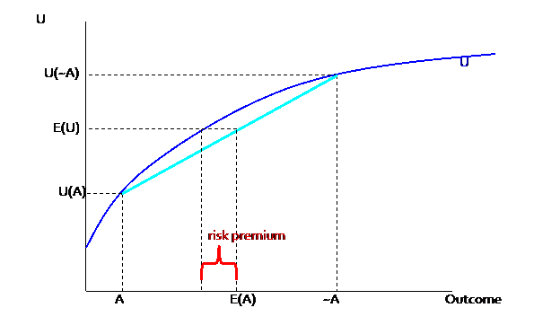
Often is convenient to suppose that an individual's
instantaneous utility depends on two factors, income and some other event, some
disaster. We assume that income is at
level Y no matter which of the two outcomes occurs; then the other event is
either A occurs or it does not (~A).
Then utility is ![]() or
or ![]() . Evidently if
the probability of A occurring is
. Evidently if
the probability of A occurring is ![]() then the
probability of A not occurring is
then the
probability of A not occurring is ![]() .
.
Various measures of how valuable it is, to eliminate the uncertainty.
Expected Surplus
Define V as the amount of income which a person would
sacrifice to be indifferent between having the full income and the disaster or
having less income but no disaster. This
is analogous to the Hicks measure of income effect that you learned back in
baby Micro Theory. You might recall that
this measure of income is not generally the same depending on where you start. In this case we must differentiate between
utility starting from a disaster, ![]() , and utility starting from no disaster,
, and utility starting from no disaster, ![]() . So define:
. So define:
![]() and
and
![]() .
.
So the Expected Surplus, ES, is defined as the expected value of these valuations,
![]()
Option Price
Or the option price is the amount that a person would pay now to eliminate the uncertainty, so as to be indifferent between E(U(A)) and E(U(~A)). This option price, OP, is such that
![]() .
.
Generally the option price will be larger than the Expected Surplus due to risk aversion.
Irreversibility and
Precautionary Principle
Some decisions about the environment are irreversible, whether developing a wild "untouched" natural area or climate change that melts glaciers or loss of habitat that causes extinction of species. Additionally, there may be uncertainty about the valuation of these stocks: how much is a species worth, if we haven't even studied it yet?
This is called a "real option" in corporate finance (businesses confront these questions all of the time, investing in technologies with wildly uncertain outcomes). Waiting to make a decision becomes an investment in lowering the uncertainty of the outcome. A lower level of uncertainty has a value (from finance, people regularly trade off risk versus return, choosing for example between high-risk and high-return investment strategies or lower-risk and lower-return investments). So although making a development decision today increases the return (since the reward is closer to the present), delaying it brings a benefit of less uncertainty.
Actual Behavior of
People making Choices under Uncertainty
People don't actually make choices in a way that adheres to these models; they're more complicated and irrational.
Kahneman and Tversky give these examples (from Kahneman's 2002 Nobel Lecture):
The Asian Disease
Imagine that the United States is preparing for the outbreak of an unusual Asian disease, which is expected to kill 600 people. Two alternative programs to combat the disease have been proposed. Assume that the exact scientific estimates of the consequences of the programs are as follows:
- If Program A is adopted, 200 people will be saved
- If Program B is adopted, there is a one-third probability that 600 people will be saved and a two-thirds probability that no people will be saved
Which of the two programs would you favor? Majority choose A.
Alternate Statement:
- If Program A’ is adopted, 400 people will die
- If Program B’ is adopted, there is a one-third probability that nobody will die and a two-thirds probability that 600 people will die
Which of the two programs would you favor? Majority choose B.
This is the "Framing Effect" and it has even been shown to affect the choices of experienced physician, depending whether treatments had a "90% survival rate" or "10% mortality rate".
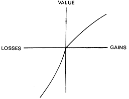
Prospect Theory
Problem 1
Would you accept this gamble?
- 50% chance to win $150
- 50% chance to lose $100
Would your choice change if your overall wealth were lower by $100?
Problem 2
Which would you choose?
lose
$100 with certainty
or
- 50% chance to win $50
- 50% chance to lose $200
Would your choice change if your overall wealth were higher by $100?
The choices are clearly identical but most people switch choices.
Can model people's utility as not from absolute level but from changes in wealth, and functional form is complicated:
"It is worth noting that an exclusive concern with the long term may be prescriptively sterile, because the long term is not where life is lived. Utility cannot be divorced from emotion, and emotion is triggered by changes. A theory of choice that completely ignores feelings such as the pain of losses and the regret of mistakes is not only descriptively unrealistic. It also leads to prescriptions that do not maximize the utility of outcomes as they are actually experienced – that is, utility as Bentham conceived it."
Most people make decisions based on simple heuristics, which are often approximately correct and are useful in minimizing the total mental effort of making a choice. Most people make choices about, say, what restaurant to choose for dinner tonight – not worth spending a great deal of time thinking about! They're not inclined to think much more deeply about bigger problems.
When college students are asked, on a survey, “How happy are you with your life in general?” and “How many dates did you have last month?” there is almost zero correlation; however if the survey asks them in the opposite order, the correlation jumps to 0.66!
The immediate corollary is that people can be cued to respond in a more statistically sound (rational or logical) manner, in ways as simple as just reminding them to "think like a statistician."
But it complicates the question of how we, as a society, ought to come to conclusions about complex issues involving a range of tradeoffs in the face of uncertain possible outcomes.
|
Hotelling on Resource Extraction |
|
|
Hotelling result on resource extraction, for an exhaustible resource, the price must grow
at a rate equivalent to the market rate of interest, so if p is the price of this resource
and r is the rate of interest then ![]() , the price will grow exponentially. Why?
, the price will grow exponentially. Why?
Arbitrage between risk-free investment (getting r) and
keeping resource in the ground. Keeping
resource in the ground returns ![]() , the percent increase of its price. Note that if extraction becomes more
difficult (diminishing returns) then more investment is required to get the
same rate of return so this will eventually become unprofitable, likely when
there is still some resource available.
, the percent increase of its price. Note that if extraction becomes more
difficult (diminishing returns) then more investment is required to get the
same rate of return so this will eventually become unprofitable, likely when
there is still some resource available.
|
Regulation of Pollution |
|
|
Command & Control
good because:
flexible in complex processes (law of unintended consequences)
more certainty for producers
bad because:
need so much information
low incentives for innovation
inefficient since generally violate equimarginal principle
Other refinements & policies:
subsidies might occasionally have some "bonus" or increasing returns provision, as with land use: a landowner who converts land to park gets more subsidy if it borders on an existing park; this is useful if the marginal benefits (to species habitat) are increasing in contiguous land area
from
Law & Econ, we know that 100% monitoring is inefficient, better to catch
some portion of offenders but fine them extra (see below)
could use "performance bonds" but these need careful monitoring (since generally forfeiture of bond involves lengthy legal proceedings); sometimes used on surface mining; also impose liquidity costs (extra financing needed) and open 'moral hazard' for regulators – 'pay-to -play'
|
Fees & Tradable
Permits |
|
|
A fee or tax per unit of emission is the Pigouvian solution – set the price and let firms decide. Tradable permits can give an equivalent outcome – permits are sold for a price; this price is essentially a tax.
Tradable Permits
Suppose
EPA issues L permits for pollution and each firm gets Li
Firm
emissions are ![]() and
and ![]()
Pollution,
p, is ![]() , so
, so ![]()
price
of pollution is a
So firm's total cost is
to minimize these costs set MTC=0 so
![]() therefore
therefore
![]()
thus equimarginal principle is met
if there are multiple receptor standards, all of which must be met, then firms will choose ei to meet the lowest limit
3 Results:
Equilibrium exists for any initial allocation of permits
Emissions from each source are efficient (no matter initial allocation)
If price equals marginal damage then equimarginal principle holds
Tradable Permits are usually allocated by either
- giving them away to current polluters (usually proportional to current pollution amounts, sometimes called 'grandfathering')
- auctioning them off to the highest bidder
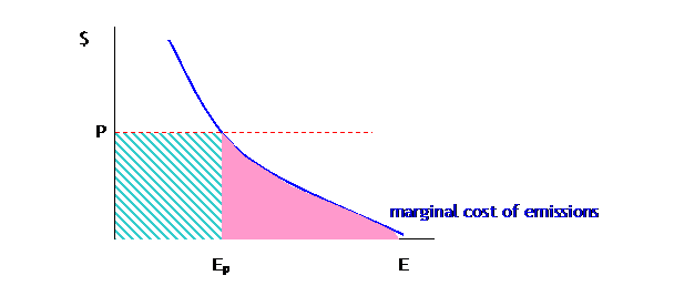
Can easily show the financial burden on firms. Consider first the simple case: tradable permits sell for a price, P. At this price the firm chooses emissions of Ep.
Because, if the firm emitted more than Ep, it could cut emissions at low cost and sell permits at a higher cost; if the firm emitted less than Ep, it is cheaper to buy permits than cut emissions itself.
If the firm were given no permits at all, it would cost
Where the pink triangle is the cost of compliance: the emissions that the firm cuts back in response to the permit regime. The striped box shows the cost of buying Ep permits at price P. If the firm were given a few permits, E1, insufficient for its needs, then it woulc face the same cost of compliance but now:
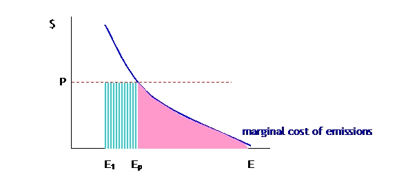
Under this regime the firm gets E1 permits and so only needs to buy the remaining permits, Ep – E1. Or the firm might even get extra permits, which could reduce its costs below the cost of compliance:
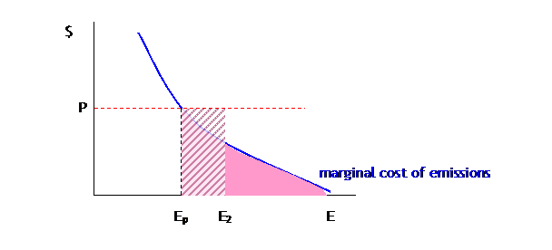
Now the firm gets E2 permits, of which it sells off (E2 – Ep) for a profit, which mitigates some of the cost of compliance.
If the permits are allocated only once (for example, when the policy is begun), then the dynamic effects of keeping unprofitable firms going (noted in the section on subsidizing firms not to pollute) will be small. If there are regular allocations of permits (yearly, for example) then these dynamic effects will be larger.
If the permits are given out in proportion to past emissions then firms will have an incentive to raise emissions just before the law goes into effect. Since many laws are debated for quite a while before taking effect, this is relevant. A law might have a multiyear lookback period.
Giving out permits in proportion to past emissions is also discriminatory to new entrants. If we consider policies like carbon permits to mitigate global climate change then this would mean that emerging economies would get fewer permits relative to richer countries.
Nonetheless giving out permits is common because it might make the program politically feasible: existing firms are given these valuable permits to get them to accept the new standards.
Further details of cap-and-trade emission control systems:
- Only optimal for uniformly distributed pollutants – CO2 leading to Global Climate Change is a perfect example
- For pollutants where the distribution is uneven, cap-and-trade could lead to more harm. If the plant with the highest cost to cleaning buys many permits, then its neighborhood will be highly polluted. However US experience with SO2 has been reasonably successful.
- For non-uniform pollutants, the trading could be moderated by transfer coefficients (below)
- Depends on all actors being profit-maximizing – many polluters are government agencies, so this assumption might be poorly fit particular cases
- If there are only a few firms, then the assumption of perfect competition becomes risible. One dominant firm could either get its permits cheaply or force competitors to pay extra.
- Transactions costs can also reduce the efficiency of the market
- So trading among zones or with complicated transfer coefficients has problems of both high transactions costs AND market power
|
When Costs & Benefits are Imperfectly Known (i.e. The Real
World…) |
|
|
Can think of regulation as either controlling quantity or price. Issuing a particular number of permits is setting the quantity and letting market determine the price of emission; a fee or tax sets the price of emission and lets the market determine quantity.
Need to consider:
§ whether there is relatively more uncertainty about marginal savings or marginal damages
§ whether marginal savings or marginal damages are relatively steep
E.g.
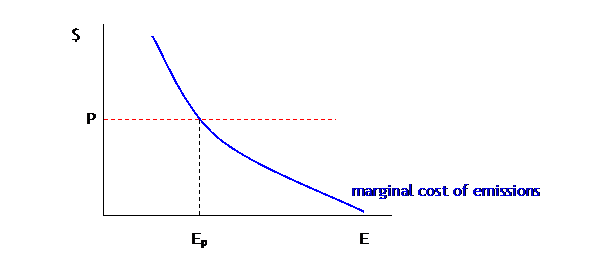
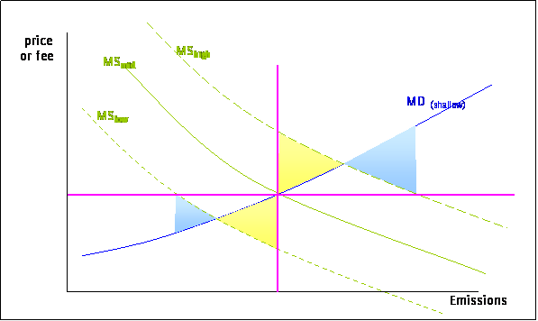
If MD known but MS uncertain,
if MD steep then quantity better (e.g. threshold effects)
if MD flat then price (emissions fees) better
If MD is steep and MS is uncertain: DWL from setting price (blue shaded areas) is large; DWL from setting quantity (yellow shaded areas) is smaller.
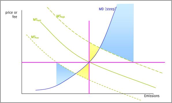
If the MD is shallow and MS is uncertain then
Regulation of Quantity, in real world, must specify:
- time of permit duration (daily, annually, etc)
- information required
- monitoring data to be provided
- inspection schedule and costs of non-compliance (review Law & Econ result)
For dynamic efficiency, price regulation can be more effective than quantity regulation since there are better incentives for innovation – the price target is known so the marginal benefit to efficiency is known, which lowers the uncertainty of investment in efficiency.
Hybrid Price/Quantity controls can be better, to replicate the marginal net social damage
|
Fees and Permits can be varied over time and place |
|
|
basic model distinguishes sources and receptors, spread over space
emissions, ei, from source any of I sources (plus background levels, B)
cause pollution, pj, at any of J receptors
![]()
linearize for each j to get transfer coefficients, ![]() (valid in
neighborhood if function is differentiable)
(valid in
neighborhood if function is differentiable)
distinguish marginal damage of receiving p versus marginal savings of emitting e
Marginal Damage Cost, MDC, then is
![]()
Firms save money by emitting freely, so Marginal Control Cost
Social
Optimum, (assume one pollutant) for each emission, i:
![]()
Pigouvian Optimal tax policy implies set ![]() therefore firms
will choose emissions such that
therefore firms
will choose emissions such that
![]() or
or ![]()
What if different firms (firms with different transfer coefficients) pay same tax? Some inefficiency; size depends on elasticity of demand
If ![]() are the optimal
amounts that emitters 1 and 2 ought to pay,
are the optimal
amounts that emitters 1 and 2 ought to pay,
but instead the tax is set at ![]() , then the DWL is:
, then the DWL is:
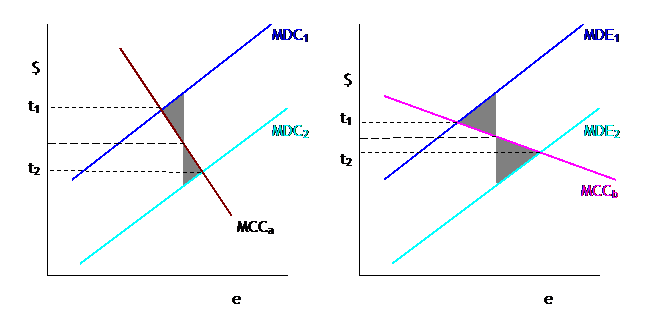
So efficiency depends on relative elasticities
again.
Over Time
This analysis is for pollution that is transitory. However much pollution is cumulative: current emissions will pollute for a lengthy time period.
Model with stock of pollutants, St, the stock at time t, increased by current emissions, et, while some fraction (d) of previous pollutants decay.
St
= dSt–1 + et
The Net Cost, NC is the present discounted value of all future costs of lowering emissions and all future damages from the stock of pollutants:
![]()
so the marginal net cost per level of emission is
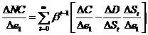
where, from ![]() , we can re-write
, we can re-write ![]() so that
so that ![]() so
so  .
.
To minimize Net Cost, NC, set Marginal Net Cost equal to
zero (the present discounted value of costs and damages equal to each other),
which implies, notating ![]() and
and ![]() , means setting
, means setting ![]() .
.
This can be interpreted as the marginal savings today should be equal to the sum of marginal damages in the future, where the future damages are discounted both by time preference and the persistence of the pollutant.
Of course for the case where the pollutant in completely transitory, so d=0, this gives us the same formula as before.
|
Regulation through Liability |
|
|
- more law & econ
Tort law (liability) involves the state setting rules to govern the behavior of 2 individuals, the injurer and the victim (technically, the potential injurer and potential victim, but for now we use the shorthand terms). Both may take a certain amount of care in their activities. For instance a manufacturer of a toy should take care that it not be dangerous; buyers should take care that it not be used in a dangerous way. Denote x as the care taken by the injurer, at a cost c(x). Often we might assume that the cost rises with x. Then denote L(x) as the loss to the victim; presumably it would be a decreasing function of x. The social objective function is to provide incentives for people to choose x to min c(x) + L(x). A typical analysis would show that the optimal level of care, x*, is where the marginal cost equals the marginal loss.
There are at least three possible sets of rules that would set incentives to each party:
- No liability would give the injurer an incentive to minimize x, without regard to L.
- Strict liability has the injurer paying all costs, so their costs are c(x) + L(x), so the injurer would take the optimal amount of care
- Negligence, where the injurer is liable for all costs if he/she did not exercise “reasonable care”. If the level of reasonable care, x’, is set equal to the optimal level, x*, then this would provide the proper incentives again. If the injurer takes less care then they are back in the “strict liability” world where they pay the full costs; if they take more care then they have no gain; so they should set x = x*.
Up to now we have discussed care as taken only by the injurer. But now introduce care by the victim, y, so again there is c(y) the cost of the victim taking care and now L(x,y), where the loss to the victim depends on the care taken by each party. Now society wants to min c(x) + c(y) + L(x,y). Now there are two optimal levels, x* and y*, that set the marginal cost of care equal to the marginal diminution of loss.
Now the liability standards are:
- No liability, so x=0 and y is too high.
- Strict liability, where now the injured party has no costs so y=0 and x is too high.
- Strict division of losses, where each side pays some fraction of the loss, f. In this case the injurer will min c(x) + fL(x,y) and so choose x to set MC(x) = f*ML, so x will be too low. Similarly for the victim, who will min c(y) + (1 – f)L(x,y) and will choose a y that is too low.
- Negligence, where the injurer is liable if their care is below some x’ value. This must be analyzed as a game, since the outcome depends on the other actor’s behavior. We can see that the Nash equilibrium has each side choosing x* and y*. Suppose that the victim chose y* and the injurer is choosing. He/she knows that if care is too low then he/she will pay the full costs, so just as in the simpler case the injurer will choose x*. The victim will face the same choice: if the injurer chooses x* then the victim will be liable for the losses if y is too low; again the victim will choose y*.
- Strict liability with defense of contributory negligence, where the injurer is fully liable unless the victim’s care was below some y’ level. Again, if y’ is set to y* then this gives an optimal outcome.
- Double liability, where each side bears the full costs. The problem with strict division was that neither side took due account of the loss. If both sides pay the full cost, however, then both will take due care. This is useful in cases where the level of care is difficult to observe. It is the logic behind “no fault” car insurance where each party’s car insurance pays the bills and the traffic courts separately determine fault.
Regulation through
Insurance
Insurance is intimately tangled with liability since often a firm, which is legally liable for some action, will buy insurance against that outcome (for instance, Director's & Officer's Insurance, which covers the company management from personal liability for their decisions at work). Workman's compensation is often used to cover liability to hazardous working conditions.
Insurance, to work well, needs six factors:
- risk pooling of
- clear losses
- over a well-defined time period
- that are frequent enough
- with a small moral hazard and
- small problems of adverse selection.
Note that "pooling" problems gave rise to reinsurance.
|
Valuation of Life |
|
|
See Viscusi (1993) "The Value of Risks to Life and Health," Journal of Economic Literature.