|
Lecture Notes 4 Supplement Cost
Curves Economics of the
Environment and Natural Resources/Economics of Sustainability K Foster, CCNY, Spring 2011 |
|
|
Cobb Douglas Example
Consider a numerical example of a firm with a very simple
Cobb-Douglas production function, so ![]() so the marginal
products are
so the marginal
products are  (the last
equation comes from a convenient simplification; it's a bit of a trick that's
not obvious the first time you see it but you should be able to verify that it
is, indeed, correct) and
 ![]() . The firm's
cost is
. The firm's
cost is ![]() So put these
expressions for the marginal products into the firm's marginal conditions that
So put these
expressions for the marginal products into the firm's marginal conditions that ![]() so
so  so
so ![]() or
or ![]() . Put this into
the production function to solve for
. Put this into
the production function to solve for  so
so  and
and  -- these are
the input demand functions, giving the firm's demand for each input as a
function of both its output level and the relative price of the input. Put these into the cost function to find
that the long-run cost is
 ![]() .
.
The long-run average cost is thus ![]() which sets the
price in the market.
which sets the
price in the market.
This allows us to easily see the scale and substitution effects. If the cost of an input, say w1,
rises, then this will mean that directly less of that input is used since  ; this is the substitution effect. However it also raises the firm's average
costs,
 ![]() in the long run
so the amount sold must decrease. The
size of this decrease in output depends on demand elasticity: if the output is
elastically demanded then the price rise will produce a sizeable downward shift
in quantity demanded.
in the long run
so the amount sold must decrease. The
size of this decrease in output depends on demand elasticity: if the output is
elastically demanded then the price rise will produce a sizeable downward shift
in quantity demanded.
Costs
The cost function is ![]() . It is
determined, in the long run, by the wages of each input and by the level of
output chosen. In the short run it is
also determined by the amount of the fixed factor.
. It is
determined, in the long run, by the wages of each input and by the level of
output chosen. In the short run it is
also determined by the amount of the fixed factor.
Marginal Cost is
the change in cost per change in output, ![]() . Marginal cost
is not generally constant but is commonly considered to vary with output.
. Marginal cost
is not generally constant but is commonly considered to vary with output.
We define several other costs:
Average cost, AC,
is the cost per unit of output, ![]() . In the short
run, some costs are fixed (F) and some are variable (
. In the short
run, some costs are fixed (F) and some are variable (![]() .
.
Average variable cost,
AVC, is the variable cost per unit of output, ![]() .
.
Average fixed cost, AFC, is ![]() , but since F does not change, this is just a
rectangular hyperbola and doesn’t change much – so we rarely pay much attention
to AFC. However we note that AC = AVC +
AFC.
, but since F does not change, this is just a
rectangular hyperbola and doesn’t change much – so we rarely pay much attention
to AFC. However we note that AC = AVC +
AFC.
Also, from the definition of marginal cost and of fixed
cost, we note that there is no need to define both marginal total cost and
marginal variable cost – since fixed costs don’t change, marginal fixed costs
are always zero so marginal total cost and marginal variable cost are always
identical: ![]() .
.
These SR curves are typically graphed as:

Where we note that MC must intersect AC at the minimum point of AC; also MC must intersect AVC at the minimum point of AVC. To show this, note that by definition if MC>AC then AC must rise; if MC<AC then AC must fall. The minimum point of AC is where it turns from falling to rising, where it, for at least a short (infinitesimal) time it is neither rising nor falling so MC=AC. Same argument goes for AVC.
In the long run, there are no fixed costs, so long-run average costs (LRAC) are equal to long-run variable costs. LRMC are defined analogously to the short run.
LRAC can never be greater than the short-run AC curves – having more choices can never hurt profits!
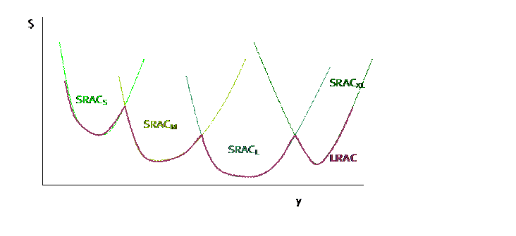
In Long Run there are no fixed costs (can always choose zero output at zero cost). LR AC curve is envelope of SR AC curves – with a scalloped edge if there are discrete plant sizes but, as plant sizes become continuously variable, the LRAC becomes a smooth curve.
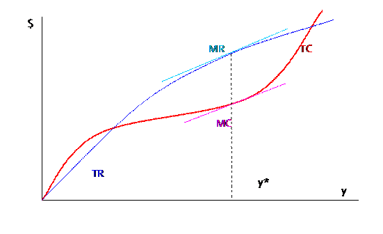
To maximize profit the firm will set ![]() . Consider this
graph, where MR is allowed to vary as well as MC. To maximize profits, the firm wants to find
where TR is farthest away from TC. The
usual argument applies: making and selling one more unit of output raises
revenue by MR; making one more unit of output raises costs by MC. If MR>MC then this was a good choice for
the firm and it should raise output more.
If MR<MC then this increased output was not a good choice and it should
decrease output. It will stop this
changing and reach equilibrium where MR=MC.
In perfect competition where P=MR, this gives us the equilibrium
condition P=MR=MC.
. Consider this
graph, where MR is allowed to vary as well as MC. To maximize profits, the firm wants to find
where TR is farthest away from TC. The
usual argument applies: making and selling one more unit of output raises
revenue by MR; making one more unit of output raises costs by MC. If MR>MC then this was a good choice for
the firm and it should raise output more.
If MR<MC then this increased output was not a good choice and it should
decrease output. It will stop this
changing and reach equilibrium where MR=MC.
In perfect competition where P=MR, this gives us the equilibrium
condition P=MR=MC.
What is the firm's demand curve? In a perfectly competitive environment the firm's demand curve is a horizontal line – the market price for this homogenous commodity. The firm can sell as much quantity as it can produce at that price. Lowering the price will not increase the amount sold; raising the price will stop all sales. This is an extreme assumption but, as you think about it, not completely unrealistic. One of the important points of any business plan for a new company is 'the competition' – what other firms sell and at what price. If my firm offers the same product then I can't charge a higher price. Of course my firm might charge a higher price and offer a better product, but this means that I'm selling a different output. Sometimes I take a cab after class: whether I take a yellow cab with a meter or a black cab without, the price is the same (even though, for the latter case, it is negotiated at the end of the ride).
The business press sometimes discusses the "commodification" of different markets: for example at one point, when computers were new, the chips were quite different and there were many different prices; now that chips are standardized there is much less variability in price. Financial markets are commodity markets: nobody offers a "20% sale" on stocks or bonds! Markets are organized in order to standardize and "commoditize" certain products: e.g. the CBOT offers corn futures to deliver "5000 bushels of No. 2 yellow corn"; or "100 troy ounces of refined gold not less than .995 fineness cast as one bar or 3 one-kilogram bars"; the NYMEX trades gasoline "reformulated gasoline blendstock for oxygen blending (RBOB) futures contract trade in units of 42,000 gallons (1,000 barrels)" for delivery in New York; Fannie Mae creates bundles of home mortgages that are created to be homogenous (each mortgage has a specified list of criteria).
This is not to say that the market demand curve is flat, just that the curve for the particular firm is flat. Another way of thinking of it is that the firm is such a tiny player in the whole market that it sees just a tiny piece of it, which is essentially flat. But even if there are a limited number of companies then a firm might still face a flat demand curve for its product based on the other's price. A final example: whatever I sell nowadays, I have to know what Amazon or eBay charges for it – that (plus shipping) is the highest price I can charge!
Profit Maximization
in the Short Run
In the short run the firm must account separately for fixed
costs. The profit maximization becomes: ![]() . Note that
variable costs,
. Note that
variable costs, ![]() , are a function of the level of output but
"Fixed Costs are fixed." Fixed
Costs don't change depending on the level of output, they're fixed. So the lowest level of profits that the firm
could make are
, are a function of the level of output but
"Fixed Costs are fixed." Fixed
Costs don't change depending on the level of output, they're fixed. So the lowest level of profits that the firm
could make are ![]() if output is
set to zero (revenue and variable cost both become zero in that case). Beyond this, however, the usual rules
apply. Recall that the marginal variable
cost is exactly equal to marginal total cost.
MC is how much cost increases when output increases. MR (which we assume to be
if output is
set to zero (revenue and variable cost both become zero in that case). Beyond this, however, the usual rules
apply. Recall that the marginal variable
cost is exactly equal to marginal total cost.
MC is how much cost increases when output increases. MR (which we assume to be ![]() in this case,
for simplicity) is the amount by which revenue increases when output
rises. Again, if MR>MC then the firm
will produce more; if MR<MC then less.
in this case,
for simplicity) is the amount by which revenue increases when output
rises. Again, if MR>MC then the firm
will produce more; if MR<MC then less.
So a firm with these cost curves (which we describe as canonical):

could face prices that lie in 3 separate regions: (A) either price intersects MC where MC is above AC; or (B) price intersects MC where MC is below AC but above AVC; or (C) price intersects MC where MC is below AVC.
Consider (A):
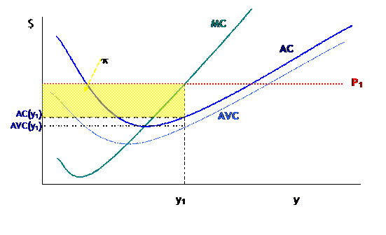
in this case, when price is at P1, the firm will
choose y1 level of output to maximize profits. Profits are ![]() but can be
more easily seen graphically as
but can be
more easily seen graphically as ![]() . So profits
are drawn as the area of the rectangle with height
. So profits
are drawn as the area of the rectangle with height ![]() and width
and width ![]() , marked yellow in the graph. The decomposition of costs into Variable Costs
and Fixed Costs can also be seen: VC are the area of the rectangle with height
, marked yellow in the graph. The decomposition of costs into Variable Costs
and Fixed Costs can also be seen: VC are the area of the rectangle with height ![]() and width
and width ![]() ; FC is the area of the rectangle with height
; FC is the area of the rectangle with height ![]() and width
and width ![]() .
.
With price at (B), where it intersects MC where MC is below AC but above AVC, we find:

Again the firm chooses the point where ![]() , which is
, which is ![]() . Profit here
is actually negative, since
. Profit here
is actually negative, since ![]() , the firm's average costs are greater than average
revenue. So the question arises, is the
firm really maximizing profit? Well,
what else could the firm do? It could
shut down completely, but in this case it would lose
, the firm's average costs are greater than average
revenue. So the question arises, is the
firm really maximizing profit? Well,
what else could the firm do? It could
shut down completely, but in this case it would lose ![]() , which, in the diagram, is again the area of the
rectangle with height
, which, in the diagram, is again the area of the
rectangle with height ![]() and width
and width ![]() -- and this
rectangle is clearly bigger than the actual profit lost. Basically, since operating costs (AVC) are
below the price, it makes sense to operate even if the firm doesn't cover all
of its fixed costs. It covers some
amount of its fixed costs and so reduces its losses. This is just another manifestation of the old
rule: sometimes the best that we can do still isn't very good. The firm is maximizing profits but still losing
money.
-- and this
rectangle is clearly bigger than the actual profit lost. Basically, since operating costs (AVC) are
below the price, it makes sense to operate even if the firm doesn't cover all
of its fixed costs. It covers some
amount of its fixed costs and so reduces its losses. This is just another manifestation of the old
rule: sometimes the best that we can do still isn't very good. The firm is maximizing profits but still losing
money.
Only in the case of (C) would the firm actually shut down. Consider:
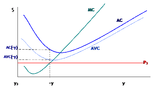
Now with price at ![]() , the firm could choose to continue producing where
, the firm could choose to continue producing where ![]() , at the point labeled
, at the point labeled ![]() (from computer
programming, the tilde means "Logical Not"). But at this point, the losses to operating,
totaling
(from computer
programming, the tilde means "Logical Not"). But at this point, the losses to operating,
totaling ![]() would be larger
than the losses to just closing down and losing fixed costs, the rectangle of
area
would be larger
than the losses to just closing down and losing fixed costs, the rectangle of
area ![]() . So the firm
chooses
. So the firm
chooses ![]() whenever the
price is less even than average variable costs.
whenever the
price is less even than average variable costs.
This tripartite division has many real-life ramifications. This is why hotels and airlines are willing to give last-minute deals: a butt in an airplane seat paying even $20 is more than the extra cost for the jet fuel to haul that little bit more weight. They try and try to charge more, to cover their fixed costs, but when it comes right down to the end they know that their variable costs are low.
Another ramification is seen in the current housing bust. Driving through certain neighborhoods, there are still houses being constructed – why? Clearly the answer is that, since the builder has bought the land (usually the most expensive part), that FC is lost now. If a house sits half-built then the construction company loses all the costs put into it so far. But even if completing the building takes more expense, it might still be worthwhile – the builders will lose money, but not as much as if they walked away.
Firm Supply Curve
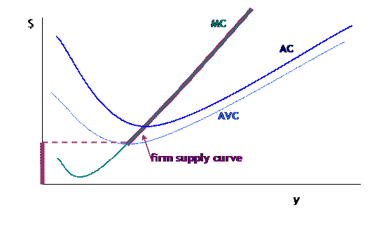
The firm's supply curve is then the locus of price and quantity choices, which is the firm's MC curve above AVC, then quantity jumps to zero if the price falls below this point. In the graph, this is:
|
Consumer Choice and
Fees/Taxes |
|
|
There may be cases where policymakers are reluctant to impose fees for worry about the distributional impacts. For example, water pricing may lead to more efficient outcomes but this could lead to the poorest people suddenly facing a steep price hike for a necessary good. A gas tax, carbon emissions permits, and other programs all have this feature.
The simple way to fix this is to rebate the tax revenue to each person (but regardless of how much was purchased). With some basic micro we can show that the increased income will stimulate spending on the good but the price rise will diminish spending – we end up with a classic micro Slutsky decomposition of substitution and income effects.
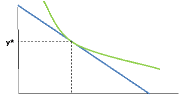
Consider a typical consumer who chooses between good X and good Y (where Y is a composite of “all other goods”). Assume the price of Y is $1 and the price of X is P. The consumer has income of M. Then her budget constraint looks like this:

y x x*
And assume she chooses the point, (X*,Y*) as indicated.
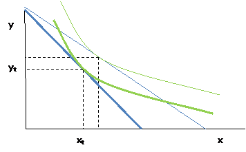
Now a tax of T on good X would result in a rise in the price of X to (P + T) and shift her budget set inward, getting her to a lower utility level:
Now suppose that some of the revenue from this tax were rebated, to raise the person's income from M to M' to make the old X*,Y* just affordable.
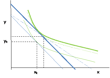
Then the person is no worse off but still is using less of the good x – through only the substitution effect not the income effect.
Further refinements could adjust the marginal prices so that, for example, the first few units are available at a low cost while remaining units are more costly. This would provide people with a minimum level of the good without substantial deleterious effects on efficiency.
|
Choice of Dumping or Safe Disposal |
|
|
( from Kolstad's
Environmental Econ textbook)
Sometimes polluters face a choice of either cheaply dumping emissions (in a way that is socially harmful) or safely disposing of them. An example is garbage – it may be optimal to try to give households incentives to reduce their garbage by charging per pound or per bin, but this might also provide incentives for people to dump garbage in some deserted area. Consumers' batteries and electronic devices should be properly disposed of. This is especially relevant for producers who use various chemicals that need proper disposal.
One option is subsidizing the safe disposal, but this is costly and, of course, encourages more disposal. Suppose households were paid some amount of money per pound or per bin of garbage! That sounds crazy – but it might not be, if we can change other costs.
Assume a firm can dispose of waste, w, either, safely at
cost ![]() or not safely
at cost
or not safely
at cost ![]() . Clearly there
is only a problem if
. Clearly there
is only a problem if ![]() . So the
government might introduce a subsidy per unit of waste, so changing the cost of
proper disposal to
. So the
government might introduce a subsidy per unit of waste, so changing the cost of
proper disposal to ![]() (if the subsidy
does not lower the cost enough then we're back to the original problem).
(if the subsidy
does not lower the cost enough then we're back to the original problem).
So how can we change other costs? Suppose the regulator observed the total
volume of waste and taxed that, so now the costs for the firm are increased by ![]() but this is
charged regardless of whether the firm dumps or disposes safely. The firm will not dispose safely if
but this is
charged regardless of whether the firm dumps or disposes safely. The firm will not dispose safely if ![]() which clearly
is no different. So the subsidy rate
should be set to give an incentive to dispose safely while the net tax on
waste,
which clearly
is no different. So the subsidy rate
should be set to give an incentive to dispose safely while the net tax on
waste, ![]() , should now equate to marginal damages.
, should now equate to marginal damages.
A classic example of this is the deposit-refund system on bottles of soda, where consumers pay extra at purchase but then get a subsidy for proper disposal.
There are other examples of narrow-focused disposal charges, where buyers initially pay more and then can claim back some of this charge if the item is properly disposed (e.g. household electronics).
|
Enforcement |
|
|
Note results from Law & Econ: if there is a probability of being caught for violations, which is less than 100%, then the fine levied will need to be larger than just the marginal damage of the pollution violation. In the risk-neutral case, the violator should be charged for the expected number of unobserved violations: if there is a 20% chance of being caught, then the penalty should be five times the size of the damage created by the firm's violation. This way the expected penalty that the polluter pays is just equal to the marginal damage (the original optimal result).
A firm can pay a penalty that has both a fixed component (D)
and a proportional component, which costs f per amount by which the firm misses
the regulated level, ![]() , which is imposed with probability p,
so the firm's total costs are its costs of production,
, which is imposed with probability p,
so the firm's total costs are its costs of production, ![]() , as well as the expected fine,
, as well as the expected fine, ![]() . This can be
graphed as a function of the level of emissions:
. This can be
graphed as a function of the level of emissions:
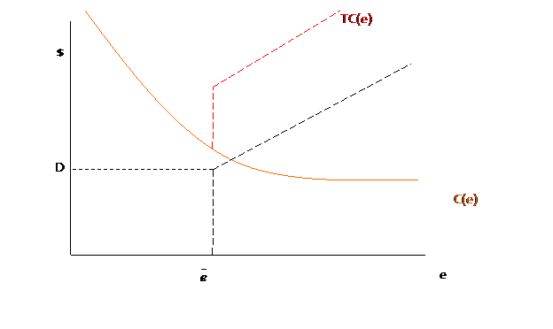
So the minimum point of TC is at the kink, ![]() . Of course
this is not infallible; the emissions level could be chosen so low, along with
a small fine, as to make only a slight change to the firm's total cost.
. Of course
this is not infallible; the emissions level could be chosen so low, along with
a small fine, as to make only a slight change to the firm's total cost.
Since enforcement comes from the expected value of the fine, pf, the regulator can save on enforcement costs by reducing p while increasing the level of the penalty, and still keep the product unchanged. There are likely to be practical limits to this, of course.
|
Cost Benefit Analysis (CBA) |
|
|
In general we want to find costs and benefits from observing people's actual market choices, but this is often impractical.
Note that private sector often does CBA but takes a smaller number of costs and benefits – only those that apply to the particular private actor. Public sector CBA takes a wider scope of costs and benefits.
If there is a market for the good or service then changes in consumer surplus or producer surplus might be a good measure. For example if pollution reduces crop yields for farmers .
Replacement cost is not quite as good but still allows getting a market-based cost.
Hedonic pricing is a fancy way of trying to infer the values that people put on various components of a purchase. For example, if you buy a house you are buying a bundle of goods: a neighborhood with various amenities from local schools to restaurants to neighbors to park access; the pollution amounts in air, water, and soil; plus the actual property (perhaps with other environmental concerns such as lead paint, asbestos, radon, …). With some fancy econometrics we should be able to establish how much, for example, people value access to a local park, by seeing how much home prices rise for good locations.
Must subdivide health risks into both mortality risk and morbidity risk, also conditional on what risks are known at the time of the purchase.
We can observe how much people spend to avert a pollutant to observe a minimum amount that a lack of pollution would be worth.
We can observe the travel costs that people incur to visit, for example, a national park, to again find a minimum valuation that they put on it.
Contingent Valuation tries to take a broad view of the amenities provided by a resource. For example if we want to find the value of a park that preserves a natural resource unspoiled, then we would separate the "Use Value" from the "Non-Use Value" and add these up to find the Total Value. Use Value is how much value people get from using the resource (sustainably or unsustainably). Non-Use Value is the value society gets from preservation. Non-Use value can be separated in turn into three components: "Option Value," "Bequest Value," and "Existence Value." Option value is the value that the resource might have in the future: a species of plant could provide a new medicine. Bequest Value notes that people value the ability to pass on certain resources to their children and grandchildren. Existence Value stems from the fact that people might value, say, the fact that there are wild lands – even if they don't visit them.
|
CS, CV & EV: Consumer Surplus, Compensating Variation
and Equivalent Variation |
|
|
Consumer Surplus
If a consumer has quasilinear preferences then the area under the demand curve is exactly the consumer surplus (the value that the consumer gets from the opportunity to trade at the market price).
Otherwise we have CV and EV – Compensating Variation or Equivalent Variation.
Both ask how much income would be required to compensate the consumer, but:
CV asks how much after the price change to get the original utility;
EV asks how much before the price change to get the later utility.
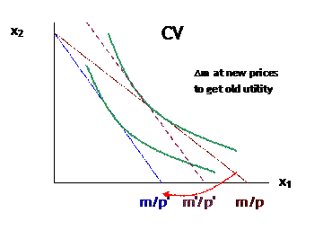
In the picture above, the price of x1 rises from p to p'. After the price change, the consumer would need m' income to get to the original indifference curve. (Note that this is the Hicks substitution effect so the addition to income would be less than the Slutsky.)
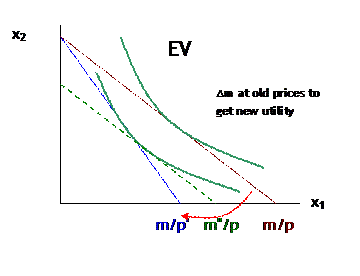
Now there is the same rise in price of x1 from p to p'. But now the consumer would need just m" to be on the later indifference curve even if the old price ratio were restored.
Examples with Cobb-Douglas preferences; comparing CV/EV.