Lecture Notes 6

Economics of the Environment and Natural Resources/Economics of Sustainability

K Foster, CCNY, Spring 2011

Tradable Permits, continued

Can easily show the financial burden on firms. Consider first the simple case: tradable permits sell for a price, P. At this price the firm chooses emissions of Ep.

Because, if the firm emitted more than E_p, it could cut emissions at low cost and sell permits at a higher cost; if the firm emitted less than E_p, it is cheaper to buy permits than cut emissions itself.

If the firm were given no permits at all, it would cost

Where the pink triangle is the cost of compliance: the emissions that the firm cuts back in response to the permit regime. The striped box shows the cost of buying Ep permits at price P. If the firm were given a few permits, E1, insufficient for its needs, then it would face the same cost of compliance but now:

Under this regime the firm gets E₁ permits and so only needs to buy the remaining permits, E_p – E₁. Or the firm might even get extra permits, which could reduce its costs below the cost of compliance:

Now the firm gets E2 permits, of which it sells off (E₂ – E_p) for a profit, which mitigates some of the cost of compliance.

If the permits are allocated only once (for example, when the policy is begun), then the dynamic effects of keeping unprofitable firms going (noted in the section on subsidizing firms not to pollute) will be small. If there are regular allocations of permits (yearly, for example) then these dynamic effects will be larger.

If the permits are given out in proportion to past emissions then firms will have an incentive to raise emissions just before the law goes into effect. Since many laws are debated for quite a while before taking effect, this is relevant. A law might have a multiyear lookback period.

Giving out permits in proportion to past emissions is also discriminatory to new entrants. If we consider policies like carbon permits to mitigate global climate change then this would mean that emerging economies would get fewer permits relative to richer countries.

Nonetheless giving out permits is common because it might make the program politically feasible: existing firms are given these valuable permits to get them to accept the new standards.

These worked really well, when US instituted tradable permits for sulfur dioxide (SO₂) in 1995 (see Schmalensee et al, Journal of Economic Perspectives 1998). They show this graphic, where the heavy line shows historical emissions per plant (sorted by level) while the light bars show actual emissions.

Clearly there was enormous variation: some plants drastically reduced emissions, far below what was required; others increased. The variation gives an idea of the scope of DWL from regulation.

Further details of cap-and-trade emission control systems:

- Only optimal for uniformly distributed pollutants – CO₂ leading to Global Climate Change is a perfect example

- For pollutants where the distribution is uneven, cap-and-trade could lead to more harm. If the plant with the highest cost to cleaning buys many permits, then its neighborhood will be highly polluted. However US experience with SO₂ has been reasonably successful.

- For non-uniform pollutants, the trading could be moderated by transfer coefficients (below)

- Depends on all actors being profit-maximizing – many polluters are government agencies, so this assumption might poorly fit particular cases

- If there are only a few firms, then the assumption of perfect competition becomes risible. One dominant firm could either get its permits cheaply or force competitors to pay extra.

- Transactions costs can also reduce the efficiency of the market

- So trading among zones or with complicated transfer coefficients has problems of both high transactions costs AND market power

When Costs & Benefits are Imperfectly Known (i.e. The Real World…)

Can think of regulation as either controlling quantity or price. Issuing a particular number of permits is setting the quantity and letting market determine the price of emission; a fee or tax sets the price of emission and lets the market determine quantity.

Need to consider:

§ whether there is relatively more uncertainty about marginal savings or marginal damages

§ whether marginal savings or marginal damages are relatively steep

E.g.

If MD known but MS uncertain,

if MD steep then quantity better (e.g. threshold effects)

if MD flat then price (emissions fees) better

If MD is steep and MS is uncertain: DWL from setting price (blue shaded areas) is large; DWL from setting quantity (yellow shaded areas) is smaller.

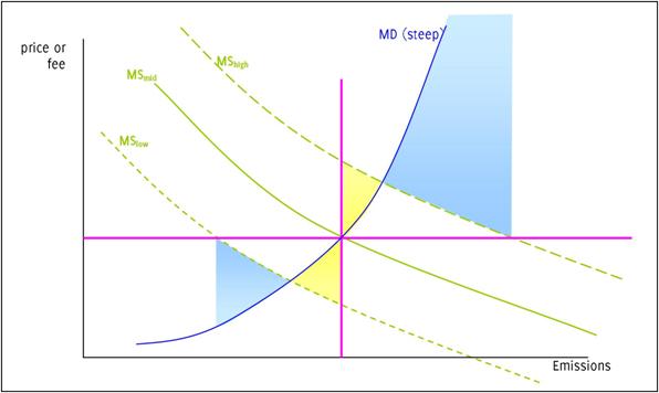
If the MD is shallow and MS is uncertain then

Regulation of Quantity, in real world, must specify:

• time of permit duration (daily, annually, etc)
• information required
• monitoring data to be provided
• inspection schedule and costs of non-compliance (review Law & Econ result)

For dynamic efficiency, price regulation can be more effective than quantity regulation since there are better incentives for innovation – the price target is known so the marginal benefit to efficiency is known, which lowers the uncertainty of investment in efficiency.

Hybrid Price/Quantity controls can be better, to replicate the marginal net social damage

Fees and Permits can be varied over time and place

basic model distinguishes sources and receptors, spread over space

emissions, e_i, from source any of I sources (plus background levels, B)

cause pollution, p_j, at any of J receptors

linearize for each j to get transfer coefficients, (valid in neighborhood if function is differentiable)

distinguish marginal damage of receiving p versus marginal savings of emitting e

Marginal Damage Cost, MDC, then is

Firms save money by emitting freely, so Marginal Control Cost

Social Optimum, (assume one pollutant) for each emission, i:

Pigouvian Optimal tax policy implies set therefore firms will choose emissions such that

or

What if different firms (firms with different transfer coefficients) pay same tax? Some inefficiency; size depends on elasticity of demand

If are the optimal amounts that emitters 1 and 2 ought to pay,

but instead the tax is set at , then the DWL is:

So efficiency depends on relative elasticities again.

Over Time

This analysis is for pollution that is transitory. However much pollution is cumulative: current emissions will pollute for a lengthy time period.

Model with stock of pollutants, St, the stock at time t, increased by current emissions, et, while some fraction (d) of previous pollutants decay.

S_t = dS_t–1 + e_t

The Net Cost, NC is the present discounted value of all future costs of lowering emissions and all future damages from the stock of pollutants:

so the marginal net cost per level of emission is

where, from , we can re-write so that so .

To minimize Net Cost, NC, set Marginal Net Cost equal to zero (the present discounted value of costs and damages equal to each other), which implies, notating and , means setting .

This can be interpreted as the marginal savings today should be equal to the sum of marginal damages in the future, where the future damages are discounted both by time preference and the persistence of the pollutant.

Of course for the case where the pollutant in completely transitory, so d=0, this gives us the same formula as before.

Regulation through Liability

- more law & econ

Tort law (liability) involves the state setting rules to govern the behavior of 2 individuals, the injurer and the victim (technically, the potential injurer and potential victim, but for now we use the shorthand terms). Both may take a certain amount of care in their activities. For instance a manufacturer of a toy should take care that it not be dangerous; buyers should take care that it not be used in a dangerous way. Denote x as the care taken by the injurer, at a cost c(x). Often we might assume that the cost rises with x. Then denote L(x) as the loss to the victim; presumably it would be a decreasing function of x. The social objective function is to provide incentives for people to choose x to min c(x) + L(x). A typical analysis would show that the optimal level of care, x*, is where the marginal cost equals the marginal loss.

There are at least three possible sets of rules that would set incentives to each party:

• No liability would give the injurer an incentive to minimize x, without regard to L.
• Strict liability has the injurer paying all costs, so their costs are c(x) + L(x), so the injurer would take the optimal amount of care
• Negligence, where the injurer is liable for all costs if he/she did not exercise “reasonable care”. If the level of reasonable care, x’, is set equal to the optimal level, x*, then this would provide the proper incentives again. If the injurer takes less care then they are back in the “strict liability” world where they pay the full costs; if they take more care then they have no gain; so they should set x = x*.

Up to now we have discussed care as taken only by the injurer. But now introduce care by the victim, y, so again there is c(y) the cost of the victim taking care and now L(x,y), where the loss to the victim depends on the care taken by each party. Now society wants to min c(x) + c(y) + L(x,y). Now there are two optimal levels, x* and y*, that set the marginal cost of care equal to the marginal diminution of loss.

Now the liability standards are:

• No liability, so x=0 and y is too high.
• Strict liability, where now the injured party has no costs so y=0 and x is too high.
• Strict division of losses, where each side pays some fraction of the loss, f. In this case the injurer will min c(x) + fL(x,y) and so choose x to set MC(x) = f*ML, so x will be too low. Similarly for the victim, who will min c(y) + (1 – f)L(x,y) and will choose a y that is too low.
• Negligence, where the injurer is liable if their care is below some x’ value. This must be analyzed as a game, since the outcome depends on the other actor’s behavior. We can see that the Nash equilibrium has each side choosing x* and y*. Suppose that the victim chose y* and the injurer is choosing. He/she knows that if care is too low then he/she will pay the full costs, so just as in the simpler case the injurer will choose x*. The victim will face the same choice: if the injurer chooses x* then the victim will be liable for the losses if y is too low; again the victim will choose y*.
• Strict liability with defense of contributory negligence, where the injurer is fully liable unless the victim’s care was below some y’ level. Again, if y’ is set to y* then this gives an optimal outcome.
• Double liability, where each side bears the full costs. The problem with strict division was that neither side took due account of the loss. If both sides pay the full cost, however, then both will take due care. This is useful in cases where the level of care is difficult to observe. It is the logic behind “no fault” car insurance where each party’s car insurance pays the bills and the traffic courts separately determine fault.

Regulation through Insurance

Insurance is intimately tangled with liability since often a firm, which is legally liable for some action, will buy insurance against that outcome (for instance, Director's & Officer's Insurance, which covers the company management from personal liability for their decisions at work). Workman's compensation is often used to cover liability to hazardous working conditions.

Insurance, to work well, needs six factors:

- risk pooling of

- clear losses

- over a well-defined time period

- that are frequent enough

- with a small moral hazard and

- small problems of adverse selection.

Note that "pooling" problems gave rise to reinsurance.

Valuation of Life

See Viscusi (1993) "The Value of Risks to Life and Health," Journal of Economic Literature.