|
Lecture Notes 10 Econ 20150, Principles of Statistics Kevin R Foster, CCNY Spring 2012 |
|
|
|
Regression to the Mean – OLS |
|
|
Example in class.
The example is due to Kahneman, who describes having subjects toss two coins at a target.
Here is the result:
Note that the toss of blue and red chips (blue first, then red) exhibits regression towards the mean. Does this imply learning? (You can reverse the axes, put up a regression line showing that the second toss predicts the first...)
Kahneman also gives this example (discuss):
"Highly intelligent women tend to marry men who are less intelligent than they are."
|
Jumping into OLS |
|
|
(Chapter 12 of textbook)
Learning Outcomes (from CFA exam Study Session 3, Quantitative Methods)
Students will be able to:
§ use a statistical analysis computer program to run regression
§ differentiate between the dependent and independent variables
§ explain the assumptions underlying linear regression and interpret the regression coefficients
§ calculate and interpret the standard error of estimate and a confidence interval for a regression coefficient
§ differentiate between homoskedasticity and heteroskedasticity
OLS is Ordinary Least Squares, which as the name implies is ordinary, typical, common – something that is widely used (and abused) in just about every economic analysis.
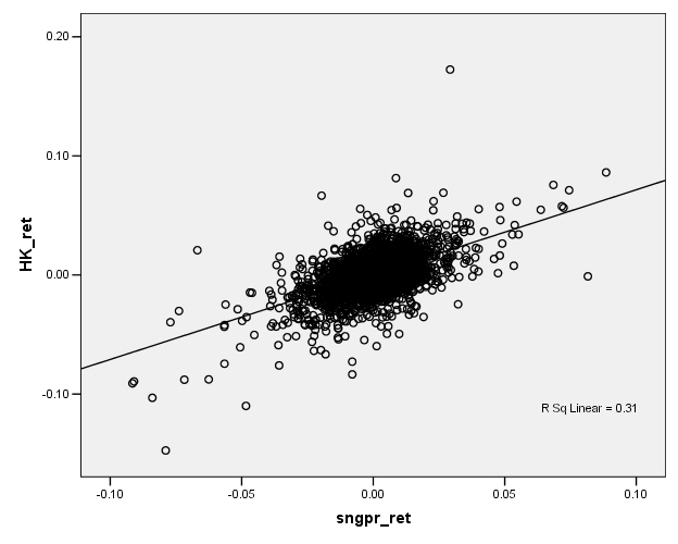
We are accustomed to looking at graphs that show values of two variables and trying to discern patterns. Consider these two graphs of financial variables.
This plots the returns of Hong Kong's Hang Seng index
against the returns of

This next graph shows the S&P 500 returns and interest rates (1-month Eurodollar) during 1989-2004.
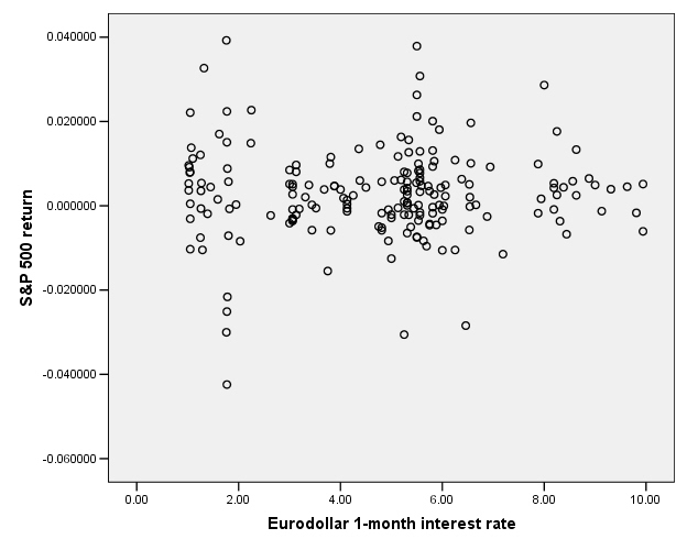
You don't have to be a highly-skilled econometrician to see
the difference in the relationships. It
would seem reasonable that the Hong Kong and
So we want to ask, how could we measure these relationships? Since these two graphs are rather extreme cases, how can we distinguish cases in the middle? How can we try to guard against seeing relationships where, in fact, none actually exist? We will consider each of these questions in turn.
How can we measure the relationship?
Facing a graph like the Hong Kong/Singapore stock indexes, we might represent the relationship by drawing a line, something like this:
Now if this line-drawing were done just by hand, just sketching in a line, then different people would sketch different lines, which would be clearly unsatisfactory. What is the process by which we sketch the line?
Typically we want to find a relationship because we want to
predict something, to find out that, if I know one variable, then how does this
knowledge affect my prediction of some other variable. We call the first variable, the one known at
the beginning, X. The variable that
we're trying to predict is called Y. So
in the example above, the
This line is drawn to get the best guess "close to" the actual Y values – where by "close to" we actually minimize the average squared distance. Why square the distance? This is one question which we will return to, again and again; for now the reason is that a squared distance really penalizes the big misses. If I square a small number, I get a bigger number. If I square a big number, I get a HUGE number. (And if I square a number less than one, I get a smaller number.) So minimizing the squared distance will mean that I am willing to make a bunch of small errors in order to reduce a really big error. This is why there is the "LS" in "OLS" -- "Ordinary Least Squares" finds the least squared difference.
A computer can easily calculate a line that minimizes the
squared distance between each Y value and the best prediction. There are also formulas for it. (We'll come back to the formulas; put a
lightning bolt here to remind us: ![]() .)
.)
For a moment consider how powerful this procedure is. A line that represents a relationship between X and Y can be entirely produced by knowing just two numbers: the y-intercept and the slope of the line. In algebra class you probably learned the equation as:
where the slope is and the y-intercept is . When then , which is the value of the line when the line intersects the Y-axis (when X is zero). The y-intercept can be positive or negative or zero. The slope is the value of , which tells how much Y changes when X changes by one unit. To find the predicted value of Y at any point we substitute the value of X into the equation. Nobel laureate Chris Sims quite simply advocates that advances in science "are discoveries of ways to compress data ... with minimal loss of information." (Macroeconomics and Methodology, 1995).
In econometrics we will typically use a different notation,
where now is the y-intercept and the slope is . (Econometricians looooove Greek letters like beta, get used to it!)
The relationship between X and Y can be positive or negative. Basic economic theory says that we expect that the amount demanded of some item will be a positive function of income and a negative function of price (for a normal good). We can easily have a case where .
If X and Y had no systematic relation, then this would imply that (in which case, is just the mean of Y). In the case, Y takes on higher or lower values independently of what is the level of X.
This is the case for the S&P 500 return and interest rates:
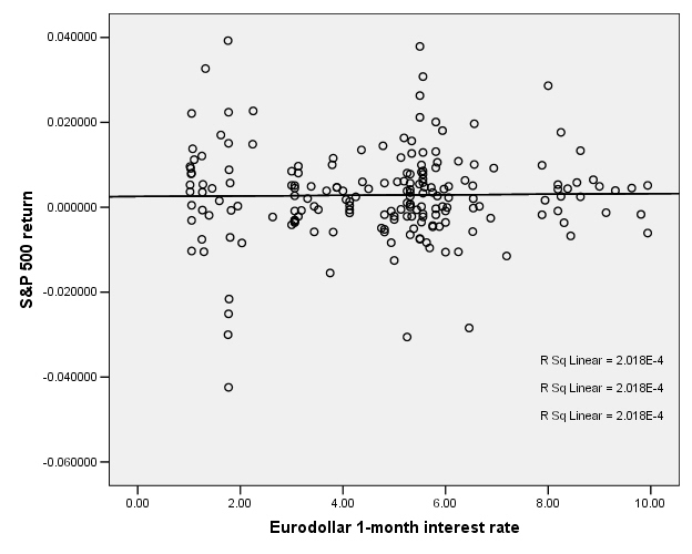
So there does not appear to be any relationship.
Sidebar:
There is another possible notation, that . This is often heard in discussions of hedge funds or financial investing. If X is the return on, say, the broad stock market (the S&P500, for example) and Y is the return of a hedge fund, then the hedge fund managers must make a case that they can provide "alpha" – that for their hedge fund . This implies that no matter what the market return is, the hedge fund will return better. The other desirable case is for a hedge fund with beta near zero – which might seem odd at first. But this provides diversification: a low beta means that the fund returns do not really depend on the broader market.
Computer programs will easily compute this OLS line; even Excel will do it. When you create an XY (Scatter) chart, then right-click on the data series, "Add Trendline" and choose "Linear" to get the OLS estimates.
Lets fine up the notation a bit more: when we fit a line to the data, we do not always have Y exactly and precisely equal to . Sometime Y is a bit bigger, sometimes a bit smaller. The difference is an error in the model. So we should actually write where epsilon is the error between the model value of Y and the actual observed value.
Another Example
This representation is powerful because it neatly and compactly summarizes a great deal of underlying variation. Consider the case of looking at the time that people spend eating and drinking, as reported in the ATUS data; we want to see if there is a relationship with the person's age. If we compute averages for each age (average time spent by people who are 18 years old, average time spent by people who are 19 years old, 20 years old, etc – all the way to 85 years old) along with the standard errors we get this chart:
There seems to be an upward trend although we might distinguish a flattening of time spent, between ages 30 and 60. But all of this information takes a table of numbers with 67 rows and 4 columns s0 268 separate numbers! If we represent this as just a line then we need just two numbers, the intercept and the slope. This also makes more effective use of the available information to "smooth out" the estimated relationship. (For instance, there is a leap up for 29-year-olds but then a leap back down – do we really believe that there is really that sort of discontinuity or do we think this could just be the randomness of the data? A fitted line would smooth out that bump.)
How can we distinguish cases in the middle?
Hopefully you've followed along so far, but are currently wondering: How do I tell the difference between the Hong Kong/Singapore case and the S&P500/Interest Rate case? Maybe art historians or literary theorists can put up with having "beauty" as a determinant of excellence, but what is a beautiful line to econometricians?
There are two separate answers here, and it's important that
we separate them. Many analyses muddle
them up. One answer is simply whether
the line tells us useful information.
Remember that we are trying to estimate a line in order to persuade
(ourselves or someone else) that there is a useful relationship here. And "useful" depends crucially upon
the context. Sometimes a variable will
have a small but vital relationship; others may have a large but much less
useful relation. To take an example from
macroeconomics, we know that the single largest component of GDP is
consumption, so consumption has a large impact on GDP. However
This first question, does the line persuade, is always contingent upon the problem at hand; there is no easy answer. You can only learn this by reading other people's analyses and by practicing on your own. It is an art form to be learned, but the second part is science.
The economist Dierdre McCloskey has a simple phrase, "How big is big?" This is influenced by the purpose of the research and the aim of discovering a relation: if we want to control some outcome or want to predict the value of some unknown variable or merely to understand a relationship.
The first question, about the usefulness and persuasiveness of the line, also depends on the relative sizes of the modeled part of Y and the error. Returning to the notation introduced, this means the relative sizes of the predictable part of Y, , versus the size of . As epsilon gets larger relative to the predictable part, the usefulness of the model declines.
The second question, about how to tell how well a line describes data, can be answered directly with statistics, and it can be answered for quite general cases.
How can we try to guard against seeing relationships where, in fact, none actually exist?
To answer this question we must think like statisticians, do mental handstands, look at the world upside-down.
Remember, the first step in "thinking like a statistician" is to ask, What if there were actually no relationship; zero relationship (so )? What would we see?
If there were no relationship then Y would be determined just by random error, unrelated to X. But this does not automatically mean that we would estimate a zero slope for the fitted line. In fact we are highly unlikely to ever estimate a slope of exactly zero. We usually assume that the errors are symmetric, i.e. if the actual value of Y is sometimes above and sometimes below the modeled value, without some oddball skew up or down. So even in a case where there is actually a zero relationship between Y and X, we might see a positive or negative slope.
We would hope that these errors in the estimated slope would be small – but, again, "how small is small?"
Let's take another example. Suppose that the true model is Y = 10 + 2X (so and ). But of course there will be an error; lets consider a case where the error is pretty large. In this case we might see a set of points like this:
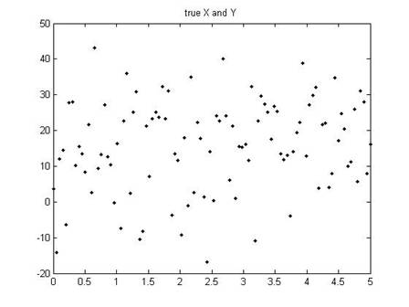
When we estimate the slope for those dots, we would find not 2 but, in this case (for this particular set of errors), 1.61813.
Now we consider a rather strange thing: suppose that there were actually zero relationship between X and Y (so that actually ). Next suppose that, even though there were actually zero relation, we tried to plot a line and so calculated our estimate of . To give an example, we would have the computer calculate some random numbers for X and Y values, then estimate the slope, and we would find 1.45097. Do it again, and we might get 0.36131. Do it 10,000 times (not so crazy, actually – the computer does it in a couple of seconds), and we'd find the following range of values for the estimated slope:
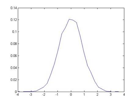
So our estimated slope from the first time, 1.61813, is "pretty far" from zero. How far? The estimated slope is farther than just 659 of those 10,000 tries, which is 6.59%.
So we could say that, if there were actually no relationship between X and Y, but we incorrectly estimated a slope, then we'd get something from the range of values shown above. Since we estimated a value of 1.61813, which is farther from zero than just 6.59% if there were actually no relationship, we might say that "there is just a 6.59% chance that X and Y could truly be unrelated but I'd estimate a value of 1.61813." [This is all based on a simple program in Matlab, emetrics1.m]
Now this is a more reasonable measure: "What is the chance that I would see the value, that I've actually got, if there truly were no relationship?" And this percentage chance is relevant and interesting to think about.
This formalization is "hypothesis testing". We have a hypothesis, for example "there is zero relation between X and Y," which we want to test. And we'd like to set down rules for making decisions so that reasonable people can accept a level of evidence as proving that they were wrong. (An example of not accepting evidence: the tobacco companies remain highly skeptical of evidence that there is a relationship between smoking and lung cancer. Despite what most researchers would view as mountains of evidence, the tobacco companies insist that there is some chance that it is all just random. They're right, there is "some chance" – but that chance is, by now, probably something less than 1 in a billion.) Most empirical research uses a value of 5% -- we want to be skeptical enough that there is only a 5% chance that there might really be no relation but we'd see what we saw. So if we went out into the world and did regressions on randomly chosen data, then in 5 out of 100 cases we would think that we had found an actual relation. It's pretty low but we still have to keep in mind that we are fallible, that we will go wrong 5 out of 100 (or 1 in 20) times.
Under some general conditions, the OLS slope coefficient will have a normal distribution -- not a standard normal, though, it doesn't have a mean of zero and a standard deviation of one.
However we can estimate its standard error and then can figure out how likely it is, that the true mean could be zero, but I would still observe that value.
This just takes the observed slope value, call it (we often put "hats" over the variables to denote that this is the actual observed value), subtract the hypothesized mean of zer0, and divide by the standard error:
We call this the "t-statistic". When we have a lot of observations, the t-statistic has approximately a standard normal distribution with zero mean and standard deviation of one.
For the careful students, note that the t-statistic actually has a t-distribution, which has a shape that depends on the number of observations used to construct it (the degrees of freedom). When the number of degrees of freedom is more than 30 (which is almost all of the time), the t-distribution is just about the same as a normal distribution. But for smaller values the t-distribution has fatter tails.
The t-statistic allows us to calculate the probability that, if there were actually a zero relationship, I might actually observe a value as extreme as . By convention we look at distance either above or below zero, so we want to know the probability of seeing a value as far from zero as either or . If were equal to 1, then this would be:
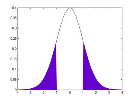
while if were another value, it would be:
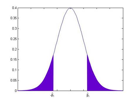
From working on the probabilities under the standard normal, you can calculate these areas for any given value of .
In fact, these probabilities are so often needed, that most computer programs calculate them automatically – they're called "p-values". The p-value gives the probability that the true coefficient could be zero but I would still see a number as extreme as the value actually observed. By convention we refer to slopes with a p-value of 0.05 or less (less than 5%) as "statistically significant".
(We can test if coefficients are different from other values than just zero, but for now that is the most common so we focus on it.)
Confidence Intervals
There is another way of looking at statistical significance. We just reviewed the procedure of taking the observed value, subtracting off the mean, dividing by the standard error, and then comparing the calculated t-statistic against a standard normal distribution.
But we could do it backwards, too. We know that the standard normal distribution has some important values in it, for example the values that are so extreme, that there is just a 5% chance that we could observe what we saw, yet the true value were actually zero. This 5% critical value is just below 2, at 1.96. So if we find a t-statistic that is bigger than 1.96 (in absolute value) then the slope would be "statistically significant"; if we find a t-statistic that is smaller than 1.96 (in absolute value) then the slope would not be "statistically significant". We can re-write these statements into values of the slope itself instead of the t-statistic.
We know from above that
,
and we've just stated that the slope is not statistically significant if:
.
This latter statement is equivalent to:
Which we can re-write as:
Which is equivalent to:
So this gives us a "Confidence Interval" – if we observe a slope within 1.96 standard errors of zero, then the slope is not statistically significant; if we observe a slope farther from zero than 1.96 standard errors, then the slope is statistically significant.
This is called a "95% Confidence Interval" because this shows the range within which the observed values would fall, 95% of the time, if the true value were zero. Different confidence intervals can be calculated with different critical values: a 90% Confidence Interval would need the critical value from the standard normal, so that 90% of the probability is within it (this is 1.64).
|
Interpretation |
|
|
In many arguments, it is important show that a certain estimator is statistically significantly different from zero. But that mere fact does not "prove" the argument and you should not be fooled into believing otherwise. It is one link in a logical chain but any chain is only as strong as its weakest link. If there is strong statistical significance then this means one link of the chain is strong, but if the rest of the argument is held together by threads it will not support any weight. As a general rule, you will rarely use a word like "prove" if you want to be precise (unless you're making a mathematical proof). Instead, phrases like "consistent with the hypothesis" or "inconsistent with the hypothesis" are better, since they remind the reader of the linkage: the statistics can strengthen or weaken the argument but they are not a substitute.
Recall the use of evidence to make an argument: if you watch a crime drama on TV you'll see court cases where the prosecutor shows that the defendant does not have an alibi for the time the crime was committed. Does that mean that the defendant is guilty? Not necessarily – only that the defendant cannot be proven innocent by demonstrating that they were somewhere else at the time of the crime.
You could find statistics to show that there is a statistically significant link between the time on the clock and the time I start lecture. Does that mean that the clock causes me to start talking? (If the clock stopped, would there be no more lecture?)
There are millions of examples. In the ATUS data, we see that people who are not working have a statistically significant increase in time on religious activities. We find a statistically significant negative correlation between the time that people spend on religious activities and their income. Do these mean that religion causes people to be poorer? (We could go on, comparing the income of people who are unusually devout, perhaps finding the average income for quartiles or deciles of time spent on religious activity.) Of course that's a ridiculous argument and no amount of extra statistics or tests can change its essentially ridiculous nature! If someone does a hundred statistical tests of increasing sophistication to show that there is that negative correlation, it doesn't change the essential part of the argument. The conclusion is not "proved" by the statistics. The statistics are "consistent with the hypothesis" or "not inconsistent with the hypothesis" that religion makes people poor. If I wanted to argue that religion makes people wealthy, then these statistics would be inconsistent with that hypothesis.
Generally two variables, A and B, can be correlated for various reasons. Perhaps A causes B; maybe B causes A. Maybe both are caused by some other variable. Or they each cause the other (circular causality). Or perhaps they just randomly seem to be correlated. Statistics can cast doubt on the last explanation but it's tough to figure out which of the other explanations is right.
|
On Sampling |
|
|
All of these statistical results, which tell us that the sample average will converge to the true expected value, are extremely useful, but they crucially hinge on starting from a random sample -- just picking some observations where the decision on which ones to pick is done completely randomly and in a way that is not correlated with any underlying variable.
For example if I want to find out data about a typical New Yorker, I could stand on the street corner and talk with every tenth person walking by – but my results will differ, depending on whether I stand on Wall Street or Canal Street or 42nd Street or 125th Street or 180th Street! The results will differ depending on whether I'm doing this on Friday or Sunday; morning or afternoon or at lunchtime. The results will differ depending on whether I sample in August or December. Even more subtly, the results will differ depending on who is standing there asking people to stop and answer questions (if the person doing the sample is wearing a formal suit or sweatpants, if they're white or black or Hispanic or Asian, if the questionnaire is in Spanish or English, etc).
In medical testing the gold standard is "randomized double blind" where, for example, a group of people all get pills but half get a placebo capsule filled with sugar while the other half get the medicine. This is because results differ, depending on what people think they're getting; evaluations differ, depending on whether the examiner thinks the test was done or not. (One study found that people who got pills that they were told were expensive reported better results than people who got pills that were said to be cheap – even though both got placebos.)
Getting a true random sample is tough. Randomly picking telephone numbers doesn't do it since younger people are more likely to have only a mobile number not a land line and poorer households may have more people sharing a single land line. Online polls aren't random (as a general rule, never believe an online poll about anything). Online reviews of a product certainly aren't random. Government surveys such as the ones we've used are pretty good – some smart statisticians worked very hard to ensure that they're a random sample. But even these are not good at estimating, say, the fraction of undocumented immigrants in a population.
There are many cases that are even subtler. This is why most sampling will start by reporting basic demographic information and comparing this to population averages. One of the very first questions to be addressed is, "Are the reported statistics from a representative sample?"
|
On Bootstrapping |
|
|
Recall the whole rationale for our method of hypothesis testing. We know that, if some average were truly zero, it would have a normal distribution (if enough observations; otherwise a t distribution) around zero. It would have some standard error (which we try to estimate). The mean and standard error are all we need to know about a normal distribution; with this information we can answer the question: if the mean were really zero, how likely would it be, to see the observed value? If the answer is "not likely" then that suggests that the hypothesis of zero mean is incorrect; if the answer is "rather likely" then that does not reject the null hypothesis.
This depends on us knowing (somehow) that the mean has a normal distribution (or a t distribution or some known distribution). Are there other ways of knowing? We could use computing power to "bootstrap" an estimate of the significance of some estimate.
This "bootstrapping" procedure was done in a previous lecture note, on polls of the household income.
Although differences in averages are distributed normally (since the averages themselves are distributed normally, and then linear functions of normal distributions are normal), we might calculate other statistics for which we don't know the distributions. Then we can't look up the values on some reference distribution – the whole point of finding Z-statistics is to compare them to a standard normal distribution. For instance, we might find the medians, and want to know if there are "big" differences between medians.
Follow the same basic procedure: take the whole dataset, treat it as if it were the population, and sample from it. Calculate the median of each sample. Plot these; the distribution will not generally have a Normal distribution but we can still calculate bootstrapped p-values.
For example, suppose I have a sample of 100 observations with a standard error equal to 1 (makes it easy; i.e. the standard error is 10 and 10/sqrt(100) = 1) and I calculate that the average is 1.95. Is this "statistically significantly" different from zero?
One way to answer this is to use the computer to create lots and lots of samples, from a population with a zero mean and standard error of 1, and then count up how many are farther from zero than 1.95. Or we can use the Standard Normal distribution to calculate the area in both tails beyond 1.95 to be 5.12%. When I bootstrapped values I got answers pretty close (within 10 bps) for 10,000 simulations. More simulations would get more precise values.
So let's try a more complicated situation. Imagine two distributions have the same mean; what is the distribution of median differences? I get this histogram of median differences:
So clearly a value beyond about 0.15 would be pretty extreme and would convince me that the real distributions do not have the same median. So if I calculated a value of -0.17, this would have a low bootstrapped p-value.
Details:
- statistical significance for a univariate regression is the same as overall regression significance – if the slope coefficient estimate is statistically significantly different from zero, then this is equivalent to the statement that the overall regression explains a statistically significant part of the data variation.
- Excel calculates OLS both as regression (from Data Analysis TookPak), as just the slope and intercept coefficients (formula values), and from within a chart
- There are important assumptions about the regression that must hold, if we are to interpret the estimated coefficients as anything other than within-sample descriptors:
o X completely specifies the causal factors of Y (nothing omitted)
o X causes Y in a linear manner
o errors are normally distributed
o errors have same variance even at different X (homoskedastic not heteroskedastic)
o errors are independent of each other
- Because OLS squares the residuals, a few oddball observations can have a large impact on the estimated coefficients, so must explore
![]() Points:
Points:
Calculating the OLS Coefficients
The formulas for the OLS coefficients have several different ways of being written. For just one X-variable we can use summation notation (although it's a bit tedious). For more variables the notation gets simpler by using matrix algebra.
The basic problem is to find estimates of b0 and b1 to minimize the error in .
The OLS coefficients are found from minimizing the sum of squared errors, where each error is defined as so we want to . If you know basic calculus then you understand that you find the minimum point by taking the derivative with respect to the control variables, so differentiate with respect to b0 and b1. After some tedious algebra, find that the minimum value occurs when we use and , where:
.
With some linear algebra, we define the equations as , where y is a column vector, , e is the same, , X is a matrix with a first column of ones and then columns of each X variable, , where there are k columns, and then . The OLS coefficients are then given as .
But the computer does the calculations so you only need these if you go on to become an econometrician.
To Recap:
- A zero slope for the line is saying that there is no relationship.
- A line has a simple equation, that Y = b0 + b1X
- How can we "best" find a value of b?
- We know that the line will not always fit every point, so we need to be a bit more careful and write that our observed Y values, Yi (i=1, …, N), are related to the X values, Xi, as: Yi = b0 + b1Xi + ui. The ui term is an error – it represents everything that we haven't yet taken into consideration.
- Suppose that we chose values for b0 and b1 that minimized the squared values of the errors. This would mean . This will generally give us unique values of b (as opposed to the eyeball method, where different people can give different answers).
- The b0 term is the intercept and the b1 term is the slope, .
- These values of b are the Ordinary Least Squares (OLS) estimates. If the Greek letters denote the true (but unknown) parameters that we're trying to estimate, then denote and as our estimators that are based on the particular data. We denote as the predicted value of what we would guess Yi would be, given our estimates of b0 and b1, so that .
- There are formulas that help people calculate and (rather than just guessing numbers); these are:
and
so that and
- Why OLS? It has a variety of desirable properties, if the data being analyzed satisfy some very basic assumptions. Largely because of this (and also because it is quite easy to calculate) it is widely used in many different fields. (The method of least squares was first developed for astronomy.)
- OLS requires some basic assumptions:
- The conditional distribution of ui given Xi has a mean of zero. This is a complicated way of saying something very basic: I have no additional information outside of the model, which would allow me to make better guesses. It can also be expressed as implying a zero correlation between Xi and ui. We will work up to other methods that incorporate additional information.
- The X and Y are i.i.d. This is often not precisely true; on the other hand it might be roughly right, and it gives us a place to start.
- Xi and ui have fourth moments. This is technical and broadly true, whenever the X and Y data have a limit on the amount of variation, although there might be particular circumstances where it is questionable (sometimes in finance).
- These assumptions are costly; what do they buy us? First, if true then the OLS estimates are distributed normally in large samples. Second, it tells us when to be careful.
- Must distinguish between dependent and independent variables (no simultaneity).
- So if these are true then the OLS are unbiased and consistent. So and . The normal distribution, as the sample gets large, allows us to make hypothesis tests about the values of the betas. In particular, if you look back to the "eyeball" data at the beginning, you will recall that a zero value for the slope, b1, is important. It implies no relationship between the variables. So we will commonly test the estimated values of b against a null hypothesis that they are zero.
- There are formulas that you can use, for calculating the standard errors of the b estimates, however for now there's no need for you to worry about them. The computer will calculate them. (Also note that the textbook uses a more complicated formula than other texts, which covers more general cases. We'll talk about that later.)
- Hypotheses about regression coefficients: t-stats, p-values, and confidence intervals again! Usually two-sided (rarely one-sided).
- Interpretation if X is a binary variable, a dummy, Di, equal to either one or zero. So the model is can be expressed as . So this is just saying that Y has mean b0 + b1 in some cases and mean b0 in other cases. So b1 is interpreted as the difference in mean between the two groups (those with D=1 and those with D=0). Since it is the difference, it doesn't matter which group is specified as 1 and which is 0 – this just allows measurement of the difference between them.
- So regression can give same info as ANOVA
- Other 'tricks' of time trends (& functional form)
- If the X-variable is just a linear change [for example, (1,2,3,...25) or (1985, 1986,1987,...2010)] then regressing a Y variable on this is equivalent to taking out a linear trend: the errors are the deviations from this trend.
- examine errors to check functional form – e.g. height as a function of age works well for age < 12 but then breaks down
- plots of x vs. (y and predicted-y) are useful as are plots of x vs e (note how to do these in SPSS)
- In addition to the standard errors of the slope and intercept estimators, the regression line itself has a standard error. One of the most commonly used is the R2 (displayed on the charts at the beginning automatically by SPSS). This is the fraction of the variance in Y that is explained by the model so 0 £ R2 £ 1. Like ANOVA. Bigger is usually better, although different models have different expectations (i.e. it's graded on a curve).