|
Lecture Notes 2 Econ 29000, Principles of Statistics Kevin R Foster, CCNY Spring 2012 |
|
|
On using these Lecture Notes:
We sometimes don't realize the real reason why our good habits work. In the case of taking notes during lecture, this is probably the case. You're not writing it, in order to have some information later. If you took your day's notes, ripped them into shreds, and threw them away, you would still learn the material much better than if you hadn't taken notes. The process of listening, asking "what are the important things said?," answering this, then writing out the answer in your own words – that's what's important! So even though I give out lecture notes, don't stop taking notes during class. Notes are not just – are not primarily! – a way to capture the fleeting knowledge that the instructor just said, before the information vanishes. Instead they are a way to process the information in a more thorough and more profound way. So keep on taking notes, even if it seems ridiculous. The reason for note-taking is to take in the material, put it into your own words, and output it. That's learning.
Two Variables
In a case where we have two variables, X and Y, we want to know how or if they are related, so we use covariance and correlation.
Suppose we have a simple case where X has a two-part distribution that depends on another variable, Y. Suppose that Y is what we call a "dummy" variable: it is either a one or a zero but cannot have any other value. (Dummy variables are often used to encode answers to simple "Yes/No" questions where a "Yes" is indicated with a value of one and a "No" corresponds with a zero. Dummy variables are sometimes called "binary" or "logical" variables.) X might have a different mean depending on the value of Y.
There are millions of examples of different means between two groups. GPA might be considered, with the mean depending on whether the student is a grad or undergrad. Or income might be the variable studied, which changes depending on whether a person has a college degree or not. You might object: but there are lots of other reasons why GPA or income could change, not just those two little reasons – of course! We're not ruling out any further complications; we're just working through one at a time.
In the PUMS data, X might be "wage and salary income in past 12 months" and Y would be male or female. Would you expect that the mean of X for men is greater or less than the mean of X for women?
Run this on SPSS ...
In a case where X has two distinct distributions depending on whether the dummy variable, Y, is zero or one, we might find the sample average for each part, so calculate the average when Y is equal to one and the average when Y is zero, which we denote . These are called conditional means since they give the mean, conditional on some value.
In this case the value of is the same as the average of .
.
This is because the value of anything times zero is itself zero, so the term drops out. While it is easy to see how this additional information is valuable when Y is a dummy variable, it is a bit more difficult to see that it is valuable when Y is a continuous variable – why might we want to look at the multiplied value, ?
Use Your Eyes
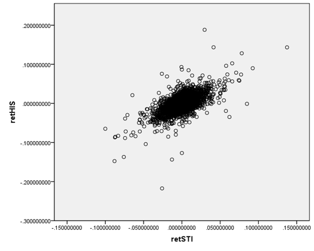
We are accustomed to looking at graphs that show values of two variables and trying to discern patterns. Consider these two graphs of financial variables.
This plots the returns of Hong Kong's Hang Seng index
against the returns of
This next graph shows the S&P 500 returns and interest rates (1-month Eurodollar) during Jan 2, 1990 – Sept 1, 2010.
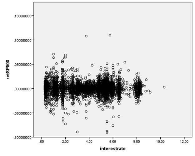
You don't have to be a highly-skilled econometrician to see
the difference in the relationships. It
would seem reasonable to state that the Hong Kong and
We want to ask, how could we measure these relationships? Since these two graphs are rather extreme cases, how can we distinguish cases in the middle? And then there is one farther, even more important question: how can we try to guard against seeing relationships where, in fact, none actually exist? The second question is the big one, which most of this course (and much of the discipline of statistics) tries to answer. But start with the first question.
How can we measure the relationship?
Correlation measures how/if two variables move together.
Recall from above that we looked at the average of when Y was a dummy variable taking only the values of zero or one. Return to the case where Y is not a dummy but is a continuous variable just like X. It is still useful to find the average of even in the case where Y is from a continuous distribution and can take any value, . It is a bit more useful if we re-write X and Y as differences from their means, so finding:
.
This is the covariance, which is denoted cov(X,Y) or sXY.
|
A positive covariance shows that when X is above its mean, Y tends to also be above its mean (and vice versa) so either a positive number times a positive number gives a positive or a negative times a negative gives a positive.
A negative covariance shows that when X is above its mean, Y tends to be below its mean (and vice versa). So when one is positive the other is negative, which gives a negative value when multiplied.
|
A bit of math (extra): = = = = =
(a strange case because it makes FOIL look like just FL!) |
Covariance is sometimes scaled by the standard deviations of X and Y in order to eliminate problems of measurement units, so define the correlation as:
or Corr(X,Y),
where the Greek letter "rho" denotes the correlation coefficient. With some algebra you can show that ρ is always between negative one and positive one; .
Two variables will have a perfect correlation if they are identical; they would be perfectly inversely correlated if one is just the negative of the other (assets and liabilities, for example). Variables with a correlation close to one (in absolute value) are very similar; variables with a low or zero correlation are nearly or completely unrelated.
Sample covariances and sample correlations
Just as with the average and standard deviation, we can estimate the covariance and correlation between any two variables. And just as with the sample average, the sample covariance and sample correlation will have distributions around their true value.
Go back to the case of the Hang Seng/Straits Times stock indexes. We can't just say that when one is big, the other is too. We want to be a bit more precise and say that when one is above its mean, the other tends to be above its mean, too. We might additionally state that, when the standardized value of one is high, the other standardized value is also high. (Recall that the standardized value of one variable, X, is , and the standardized value of Y is .)
Multiplying the two values together, , gives a useful indicator since if both values are positive then the multiplication will be positive; if both are negative then the multiplication will again be positive. So if the values of ZX and ZY are perfectly linked together then multiplying them together will get a positive number. On the other hand, if ZX and ZY are oppositely related, so whenever one is positive the other is negative, then multiplying them together will get a negative number. And if ZX and ZY are just random and not related to each other, then multiplying them will sometimes give a positive and sometimes a negative number.
Sum up these multiplied values and get the (population) correlation, .
This can be written as . The population correlation between X and Y is denoted ; the sample correlation is . Again the difference is whether you divide by N or (N – 1). Both correlations are always between -1 and +1; .
We often think of drawing lines to summarize relationships; the correlation tells us something about how well a line would fit the data. A correlation with an absolute value near 1 or -1 tells us that a line (with either positive or negative slope) would fit well; a correlation near zero tells us that there is "zero relationship."
The fact that a negative value can infer a relationship might seem surprising but consider for example poker. Suppose you have figured out that an opponent makes a particular gesture when her cards are no good – you can exploit that knowledge, even if it is a negative relationship. In finance, if a fund manager finds two assets that have a strong negative correlation, that one has high returns when the other has low returns, then again this information can exploited by taking offsetting positions.
When working with many variables we commonly create a "covariance matrix"; the matrix shows the covariance (or correlation) between each pair. So if you have 4 variables, named (unimaginatively) X1, X2, X3, and X4, then the covariance matrix would be:
|
|
X1 |
X2 |
X3 |
X4 |
|
X1 |
s11 |
|
|
|
|
X2 |
s21 |
s22 |
|
|
|
X3 |
s31 |
s32 |
s33 |
|
|
X4 |
s41 |
s42 |
s34 |
s44 |
Where the matrix is "lower triangular" because cov(X,Y)=cov(Y,X) [return to the formulas if you're not convinced] so we know that the upper entries would be equal to their symmetric lower-triangular entry (so the upper triangle is left blank since the entries would be redundant). And we can also show [again, a bit of math to try on your own] that cov(X,X) = var(X) so the entries on the main diagonal are the variances.
Depending on the application, sometimes the diagonal entries are standard errors; sometimes the correlations are given instead of covariances.
If we have a lot of variables (15 or 20) then the covariance matrix can be an important way to easily show which ones are tightly related and which ones are not.
As a practical matter, sometimes perfect (or very high) correlations can be understood simply by definition: a survey asking "Do you live in a city?" and "Do you live in the countryside?" will get a very high negative correlation between those two questions. A firm's Assets and Liabilities ought to be highly correlated. Other correlations can be caused by the nature of the sampling.
Higher Moments
The third moment is usually measured by skewness, which is a common characteristic of financial returns: there are lots of small positive values balanced by fewer but larger negative values. Two portfolios could have the same average return and same standard deviation, but if one is not symmetric (so has a non-zero skewness) then it would be important to understand this risk.
The fourth moment is kurtosis, which measures how fat the tails are, or how fast the probabilities of extreme values die off. Again a risk manager of a financial portfolio, for example, would be interested in understanding the differences between a distribution with low kurtosis (so lots of small changes) versus a distribution with high kurtosis (a few big changes).
If these measures are not perfectly clear to you, don't get frustrated – it is difficult, but it is also very rewarding. As the Financial Crisis showed, many top risk managers at name-brand institutions did not understand the statistical distributions of the risks that they were taking on. They plunged the global economy into recession and chaos because of it.
These are called "moments" to reflect the origin of the average as being like weights on a lever or "moment arm". The average is the first moment, the variance is the second, skewness is third, kurtosis is fourth, etc. If you take a class using Calculus to go through Probability and Statistics, you will learn moment-generating functions.
We usually want to know not just about correlation but also about causation, but those are not the same thing. The problem can be stated, using logical terminology, that correlation does not imply causation, but causation does imply correlation. We observe only correlations, though. Many examples...
More examples of correlation:
It is common in finance to want to know the correlation between returns on different assets.
First remember the difference between the returns and the level of an asset or index!
An investment in multiple assets, with the same return but that are uncorrelated, will have the same return but with less overall risk. We can show this on Excel; first we'll do random numbers to show the basic idea and then use specific stocks.
How can we create normally-distributed random numbers in Excel? RAND() gives random numbers between zero and one; NORMSINV(RAND()) gives normally distributed random numbers. (If you want variables with other distributions, use the inverse of those distribution functions.) Suppose that two variables each have returns given as 2% + a normally-distributed random number; this is shown in Excel sheet, lecturenotes3.xls
With finance data, we use the return not just the price. This is because we assume that investors care about returns per dollar not the level of the stock price.
Need to carefully pick the relevant time horizon. Some relationships might be over a short time horizon (high frequency traders exploit nanoseconds!) but others might be over quarters or years.
Important Questions:
· When we calculate a correlation, what number is "big"? Will see random errors – what amount of evidence can convince us that there is really a correlation?
· When we calculate conditional means, and find differences between groups, what difference is "big"? What amount of evidence would convince us of a difference?
To answer these, we need to think about randomness – in other perceptual problems, noise, blur.