|
Lecture Notes 7 Econ 20150,
Principles of Statistics Kevin R Foster, CCNY Spring 2012 |
|
|
Contents
- Hypothesis Testing
- Confidence Intervals
- p-values
- examples
Learning Outcomes (from CFA exam Study Session 3, Quantitative Methods)
Students will be able to:
§
construct and
interpret a confidence interval for a normally distributed random variable, and
determine the probability that a normally distributed random variable lies
inside a given confidence interval;
§
define the
standard normal distribution, explain how to standardize a random variable, and
calculate and interpret probabilities using the standard normal distribution;
§
explain the
construction of confidence intervals;
§
define a
hypothesis, describe the steps of hypothesis testing, interpret and discuss the
choice of the null hypothesis and alternative hypothesis, and distinguish
between one-tailed and two-tailed tests of hypotheses;
§
define and
interpret a test statistic, a Type I and a Type II error, and a significance
level, and explain how significance levels are used in hypothesis testing;
Hypothesis Testing
One of the principal tasks facing the statistician is to perform hypothesis tests. These are a formalization of the most basic questions that people ask and analyze every day – just contorted into odd shapes. But as long as you remember the basic common sense underneath them, you can look up the precise details of the formalization that lays on top.
The basic question is "How likely is it, that I'm being fooled?" Once we accept that the world is random (rather than a manifestation of some god's will), we must decide how to make our decisions, knowing that we cannot guarantee that we will always be right. There is some risk that the world will seem to be one way, when actually it is not. The stars are strewn randomly across the sky but some bright ones seem to line up into patterns. So too any data might sometimes line up into patterns.
A formal hypothesis sets a mathematical condition that I want to test. Often this condition takes the form of some parameter being zero for no relationship or no difference.
Statisticians tend to stand on their heads and ask: What if there were actually no relationship? (Usually they ask questions of the form, "suppose the conventional wisdom were true?") This statement, about "no relationship," is called the Null Hypothesis, sometimes abbreviated as H0. The Null Hypothesis is tested against an Alternative Hypothesis, HA.
Before we even begin looking at the data we can set down some rules for this test. We know that there is some probability that nature will fool me, that it will seem as though there is a relationship when actually there is none. The statistical test will create a model of a world where there is actually no relationship and then ask how likely it is that we could see what we actually see, "How likely is it, that I'm being fooled?"
The "likelihood that I'm being fooled" is the p-value.
For a scientific experiment we typically first choose the level of certainty that we desire. This is called the significance level. This answers, "How low does the p-value have to be, for me to accept the formal hypothesis?" To be fair, it is important that we set this value first because otherwise we might be biased in favor of an outcome that we want to see. By convention, economists typically use 10%, 5%, and 1%; 5% is the most common.
A five percent level of a test is conservative, it means that we want to see so much evidence that there is only a 5% chance that we could be fooled into thinking that there's something there, when nothing is actually there. Five percent is not perfect, though – it still means that of every 20 tests where I decide that there is a relationship there, it is likely that I'm being fooled in one of those – I'm seeing a relationship where there's nothing there.
To help ourselves to remember that we can never be truly certain of our judgment of a test, we have a peculiar language that we use for hypothesis testing. If the "likelihood that I'm being fooled" is less than 5% then we say that the data allow us to reject the null hypothesis. If the "likelihood that I'm being fooled" is more than 5% then the data do not reject the null hypothesis.
Note the formalism: we never "accept" the null hypothesis. Why not? Suppose I were doing something like measuring a piece of machinery, which is supposed to be a centimeter long. The null hypothesis is that it is not defective and so is one centimeter in length. If I measure with a ruler I might not find any difference to the eye. So I cannot reject the hypothesis that it is one centimeter. But if I looked with a microscope I might find that it is not quite one centimeter! The fact that, with my eye, I don't see any difference, does not imply that a better measurement could not find any difference. So I cannot say that it is truly exactly one centimeter; only that I can't tell that it isn't.
So too with statistics. If I'm looking to see if some portfolio strategy produces higher returns, then with one month of data I might not see any difference. So I would not reject the null hypothesis (that the new strategy is no improvement). But it is possible that the new strategy, if carried out for 100 months or 1000 months or more might show some tiny difference.
Not rejecting the null is saying that I'm not sure that I'm not being fooled. (Read that sentence again; it's not immediately clear but it's trying to make a subtle and important point.)
If you watched the NY Giants beat the 49ers in January, you saw the logic of hypothesis testing explained by the referee, Ed Hochuli, "To reverse on replay, there must me uncontroverted evidence that the ruling on the field is wrong. In other words, you have to be certain. Here, the ruling on the field stands." (When the 49ers player ran along the sideline to make a touchdown – the replay looked whether his feet went out of bounds.) Note that Hochuli does not say that the original referee call was right – only that they cannot say for sure that it was wrong.
To summarize, Hypothesis Testing asks, "What is the chance that I would see the value that I've actually got, if there truly were no relationship?" If this p-value is lower than 5% then I reject the null hypothesis of "no relationship." If the p-value is greater than 5% then I do not reject the null hypothesis of "no relationship."
The rest is mechanics.
The null hypothesis would tell that a parameter has some
particular value, say zero: ![]() ; the alternative hypothesis is
; the alternative hypothesis is ![]() . Under the
null hypothesis the parameter has some distribution (often normal), so
. Under the
null hypothesis the parameter has some distribution (often normal), so ![]() . Generally we have
an estimate for
. Generally we have
an estimate for ![]() , which is
, which is ![]() (for small
samples this inserts additional uncertainty).
So I know that, under the null hypothesis,
(for small
samples this inserts additional uncertainty).
So I know that, under the null hypothesis, ![]() has a standard
normal distribution (mean of zero and standard deviation of one). I know exactly what this distribution looks
like, it's the usual bell-shaped curve:
has a standard
normal distribution (mean of zero and standard deviation of one). I know exactly what this distribution looks
like, it's the usual bell-shaped curve:

So from this I can calculate, "What is the chance that I would see the value that I've actually got, if there truly were no relationship?," by asking what is the area under the curve that is farther away from zero than the value that the data give. (I still don't know what value the data will give! I can do all of this calculation beforehand.)
Any particular estimate of ![]() is generally
going to be
is generally
going to be ![]() . So the test
statistic is formed with
. So the test
statistic is formed with ![]() .
.
Looking at the standard normal pdf, a value of the test statistic of 1.5 would not meet the 5% criterion (go back and calculate areas under the curve). A value of 2 would meet the 5% criterion, allowing us to reject the null hypothesis. For a 5% significance level, the standard normal critical value is 1.96: if the test statistic is larger than 1.96 (in absolute value) then its p-value is less than 5%, and vice versa. (You can find critical values by looking them up in a table or using the computer.)
Sidebar: Sometimes you see people do a one-sided test, which
is within the letter of the law but not necessarily the spirit of the law
(particularly in regression formats). It
allows for less restrictive testing, as long as we believe that we know that
there is only one possible direction of deviation (so, for example, if the
sample could be larger than zero but never smaller). But in this case maybe the normal
distribution is inapplicable.
The test statistic can be transformed into measurements of ![]() or into a
confidence interval.
or into a
confidence interval.
If I know that I will reject the null hypothesis of ![]() at a 5% level
if the test statistic,
at a 5% level
if the test statistic, ![]() , is greater than 1.96 (in absolute value), then I can
change around this statement to be about
, is greater than 1.96 (in absolute value), then I can
change around this statement to be about ![]() . This says
that if the estimated value of
. This says
that if the estimated value of ![]() is less than
1.96 standard errors from zero, we cannot reject the null hypothesis. So cannot reject if:
is less than
1.96 standard errors from zero, we cannot reject the null hypothesis. So cannot reject if:
![]()
![]()
![]() .
.
This range, ![]() , is directly comparable to
, is directly comparable to ![]() . If I divide
. If I divide ![]() by its standard
error then this ratio has a normal distribution with mean zero and standard
deviation of one. If I don't divide then
by its standard
error then this ratio has a normal distribution with mean zero and standard
deviation of one. If I don't divide then
![]() has a normal
distribution with mean zero and standard deviation,
has a normal
distribution with mean zero and standard deviation, ![]() .
.
If the null hypothesis is not zero but some other number, ![]() , then under the null hypothesis the estimator would
have a normal distribution with mean of
, then under the null hypothesis the estimator would
have a normal distribution with mean of ![]() and standard error,
and standard error,
![]() . To transform
this to a standard normal would mean subtracting the mean and dividing by
. To transform
this to a standard normal would mean subtracting the mean and dividing by ![]() , so cannot reject if
, so cannot reject if ![]() , i.e. cannot reject if
, i.e. cannot reject if ![]() is within the
range,
is within the
range, ![]() .
.
Confidence Intervals
We can use the same critical values to construct a
confidence interval for the estimator, usually expressed in the form ![]() . This shows
that, for a given sample size (therefore
. This shows
that, for a given sample size (therefore ![]() , which depends on the sample size) that there is a
95% likelihood that the interval formed around a given estimator contains the
true value.
, which depends on the sample size) that there is a
95% likelihood that the interval formed around a given estimator contains the
true value.
This relates to hypothesis testing because if the confidence interval includes the null hypothesis then we cannot reject the null; if the null hypothesis value is outside of the confidence interval then we can reject the null.
Find p-values
We can also find p-values associated with a particular null
hypothesis by turning around the process outlined above. If the null hypothesis is zero, then with a
5% significance level we reject the null if ![]() is greater than
1.96 in absolute value. What if the
ratio
is greater than
1.96 in absolute value. What if the
ratio ![]() were 2 – what
is the smallest significance level that would still reject? (Check your understanding: is it more or less
than 5%?)
were 2 – what
is the smallest significance level that would still reject? (Check your understanding: is it more or less
than 5%?)
We can compute the ratio ![]() and then
convert this number to a p-value, which is the smallest significance level that
would still reject the null hypothesis (and if the null is rejected at a low
level then it would automatically be rejected at any higher levels).
and then
convert this number to a p-value, which is the smallest significance level that
would still reject the null hypothesis (and if the null is rejected at a low
level then it would automatically be rejected at any higher levels).
Type I and Type II
Errors
Whenever we use statistics we must accept that there is a likelihood of errors. In fact we distinguish between two types of errors, called (unimaginatively) Type I and Type II. These errors arise because a null hypothesis could be either true or false and a particular value of a statistic could lead me to reject or not reject the null hypothesis, H0. A table of the four outcomes is:
|
|
H0 is true |
H0 is false |
|
Do not reject H0 |
good! |
oops – Type II |
|
Reject H0 |
oops – Type I |
good! |
Our chosen significance level (usually 5%) gives the probability of making an error of Type I. We cannot control the level of Type II error because we do not know just how far away H0 is from being true. If our null hypothesis is that there is a zero relationship between two variables, when actually there is a tiny, weak relationship of 0.0001%, then we could be very likely to make a Type II error. If there is a huge, strong relationship then we'd be much less likely to make a Type II error.
There is a tradeoff (as with so much else in economics!). If I push down the likelihood of making a Type I error (using 1% significance not 5%) then I must be increasing the likelihood of making a Type II error.
Edward Gibbon notes that the emperor Valens would "satisfy his anxious suspicions by the promiscuous execution of the innocent and the guilty" (chapter 26). This rejects the null hypothesis of "innocence"; so a great deal of Type I error was acceptable to avoid Type II error.
Every email system fights spam with some sort of test: what is the likelihood that a given message is spam? If it's spam, put it in the "Junk" folder; else put it in the inbox. A Type I error represents putting good mail into the "Junk" folder; Type II puts junk into your inbox.
Examples
Let's do some examples.
Assume that the calculated average is 3, the sample standard
deviation is 15, and there are 100 observations. The null hypothesis is that the average is
zero. The standard error of the average
is ![]() . We can
immediately see that the sample average is more than two standard errors away
from zero so we can reject at a 95% confidence level.
. We can
immediately see that the sample average is more than two standard errors away
from zero so we can reject at a 95% confidence level.
Doing this step-by-step, the average over its standard error
is ![]() . Compare this
to 1.96 and see that 2 > 1.96 so we can reject. Alternately we could calculate the interval,
. Compare this
to 1.96 and see that 2 > 1.96 so we can reject. Alternately we could calculate the interval, ![]() , which is
, which is ![]() = (-2.94, 2.94), outside of which we reject the
null. And 3 is outside that
interval. Or calculate a 95% confidence
interval of
= (-2.94, 2.94), outside of which we reject the
null. And 3 is outside that
interval. Or calculate a 95% confidence
interval of ![]() , which does not contain zero so we can reject the
null. The critical value for the
estimate of 3 is 4.55% (found from Excel either 2*(1-NORMSDIST(2)) if using the standard normal
distribution or
2*(1-NORMDIST(3,0,1.5,TRUE)) if using the general normal distribution
with a mean of zero and standard error of 1.5).
, which does not contain zero so we can reject the
null. The critical value for the
estimate of 3 is 4.55% (found from Excel either 2*(1-NORMSDIST(2)) if using the standard normal
distribution or
2*(1-NORMDIST(3,0,1.5,TRUE)) if using the general normal distribution
with a mean of zero and standard error of 1.5).
If the sample average were -3, with the same sample standard deviation and same 100 observations, then the conclusions would be exactly the same.
Or suppose you find that the average difference between two
samples, X and Y, (i.e. ![]() ) is -0.0378.
The sample standard deviation is 0.357.
The number of observations is 652.
These three pieces of information are enough to find confidence
intervals, do t-tests, and find p-values.
) is -0.0378.
The sample standard deviation is 0.357.
The number of observations is 652.
These three pieces of information are enough to find confidence
intervals, do t-tests, and find p-values.
How?
First find the standard error of the average
difference. This standard error is 0.357
divided by the square root of the number of observations, so ![]() .
.
So we know (from the Central Limit Theorem) that the average has a normal distribution. Our best estimate of its true mean is the sample average, -0.0378. Our best estimate of its true standard error is the sample standard error, 0.01398. So we have a normal distribution with mean -0.0378 and standard error 0.01398.
We can make this into a standard normal distribution by adding 0.0378 and dividing by the sample standard error, so now the mean is zero and the standard error is one.
We want to see how likely it would be, if the true mean were actually zero, that we would see a value as extreme as -0.0378. (Remember: we're thinking like statisticians!)
The value of -0.0378 is ![]() = -2.70
standard deviations from zero.
= -2.70
standard deviations from zero.
From this we can either compare this against critical t-values or use it to get a p-value.
To find the p-value, we can use Excel just like in the homework assignment. If we have a standard normal distribution, what is the probability of finding a value as far from zero as -2.27, if the true mean were zero? This is 2*(1-NORMSDIST(-2.27)) = 0.6%. The p-value is 0.006 or 0.6%. If we are using a 5% level of significance then since 0.6% is less than 5%, we reject the null hypothesis of a zero mean. If we are using a 1% level of significance then we can reject the null hypothesis of a zero mean since 0.6% is less than 1%.
Or instead of standardizing we could have used Excel's other function to find the probability in the left tail, the area less than -0.0378, for a distribution with mean zero and standard error 0.01398, so 2*NORMDIST(-0.0378,0,0.01398,TRUE) = 0.6%.
Standardizing means (in this case) zooming in, moving from finding the area in the tail of a very small pdf, like this:
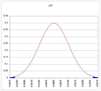
to moving to a standard normal, like this:
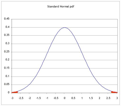
But since we're only changing the units on the x-axis, the two areas of probability are the same.
We could also work backwards. We know that if we find a standardized value greater (in absolute value) than 1.96, we would reject the null hypothesis of zero at the 5% level. (You can go back to your notes and/or HW1 to remind yourself of why 1.96 is so special.)
We found that for this particular case, each standard
deviation is of size ![]() . So we can
multiply 1.96 times this value to see that if we get a value for the mean,
which is farther from zero than 0.01398*1.96 = 0.0274, then we would reject the
null. Sure enough, our value of -0.0378
is farther from zero, so we reject.
. So we can
multiply 1.96 times this value to see that if we get a value for the mean,
which is farther from zero than 0.01398*1.96 = 0.0274, then we would reject the
null. Sure enough, our value of -0.0378
is farther from zero, so we reject.
Alternately, use this 1.96 times the standard error to find
a confidence interval. Choose 1.96 for a
95% confidence interval, so the confidence interval around -0.0378 is plus or
minus 0.0274, ![]() , which is the interval (-0.0652, -0.0104). Since this interval does not include zero we
can be 95% confident that we can reject the null hypothesis of zero.
, which is the interval (-0.0652, -0.0104). Since this interval does not include zero we
can be 95% confident that we can reject the null hypothesis of zero.
Hypothesis Testing
with two samples
In our examples we have often come up with a question where we want to know if there is a difference in mean between two groups. From the PUMS data, we could ask if, say, people in NYC are paying too much of their income to rent (where "too much" is generally defined as one-third).
For the PUMS data, SPSS tells us (using "Analyze \
Descriptive Statistics \ Descriptives") that, of
74,793 households, the average "Gross Rent as percent of income" in
the sample is 40, with a standard deviation of 28.89. So the standard error of the average is ![]() = 0.1056; so two standard errors from 40 is still only
39.7887 and 40.2113; the ideal amount of 33% of income is over 66 standard
errors away! We don't need to look up
NORMSDIST(-66) to figure that this is highly improbable. We might want to subdivide farther: to look
if the burden of rent is worse in Manhattan, say, compared with the other
boroughs.
= 0.1056; so two standard errors from 40 is still only
39.7887 and 40.2113; the ideal amount of 33% of income is over 66 standard
errors away! We don't need to look up
NORMSDIST(-66) to figure that this is highly improbable. We might want to subdivide farther: to look
if the burden of rent is worse in Manhattan, say, compared with the other
boroughs.
Now we find that in Manhattan the fraction of income going to rent is 37.79 with standard deviation of 27.608, against 41.62 (with standard error of 29.213) for the outer boroughs (SPSS output in appendix below). Are these significantly different from each other? Could we just be observing a difference that is within the range of variation that we'd expect, given such a diverse group of households? Are they statistically significantly different from each other? Our formula that we learned last time has only one n – what do we do if we have two samples?
Basically we want to figure out how to use the two separate standard errors to estimate the joint standard error; once we get that we'll use the same basic strategy to get our estimate, subtract off the null hypothesis (usually zero), and divide by its standard error. We just need to know what is that new standard error.
To do this we use the sum of the two sample variances: if we
are testing group 1 vs group 2, then a test of just
group 1 would estimate its variance as ![]() , a test of group 2 would use
, a test of group 2 would use ![]() , and a test of the group would estimate the standard
error as
, and a test of the group would estimate the standard
error as  .
.
We can make either of two assumptions: either the standard deviations are the same (even though we don't know them) or they're different (even though we don't know how different). It is more conservative to assume that they're different (i.e. don't assume that they're the same) – this makes the test less likely to reject the null.
More examples
Look at the burden of rent by household type (single vs married) in the PUMS data. (Either "Analyze \ Descriptive Statistics \ Explore" or "Analyze \ Reports \ Case Summaries" then un-click "display cases," put in "Gross Rent as percent of income" as "Variable(s)" and "Household Type" into "Grouping Variable(s)" and choose from "Statistics" to get "Number of cases," "Mean," and "Standard Deviation" to get fewer extra stats.)
|
Gross Rent as percent of income |
|||
|
Household Type |
N |
Mean |
Std. Deviation |
|
married couple |
20581 |
33.17 |
25.397 |
|
male householder no wife |
3834 |
35.42 |
26.344 |
|
female householder no husband |
15654 |
45.05 |
31.213 |
|
male householder living alone |
11520 |
41.93 |
29.555 |
|
not living alone |
3255 |
30.92 |
23.826 |
|
female householder living along |
16893 |
46.33 |
29.745 |
|
other |
3056 |
33.29 |
24.506 |
|
Total |
74793 |
40.00 |
28.893 |
The first three categories are householders (usually with families) either married (20,581 households), headed by a male (only 3834) or headed by a female (15,654 households). The remainder are living alone or in other household structures so we will ignore them for now.
Married couples have a mean rent as fraction of income as 33.17. The standard error of this mean is 25.397/sqrt(20581) = 0.178. So what is the likelihood that married couples have a mean of 33 percent of income devoted to rent, but we could observe a number as high or higher as 33.17? This is just under one standard error away. Graph this normal distribution as either:
or, standardized,
So the area in the right tail is 16.98%; the probability of seeing a difference as far away as 33.17 or farther (in either direction) is 33.96%. So we cannot reject the null hypothesis that the true value is 33% but we could observe this difference.
By contrast, the average burden of rent for female-headed households is 45.05%; this average has a standard error of 31.213/sqrt(15654) = .249. So 45.05 is 12.05 away from 33, which is (45.05 – 33)/.249 = 48.3 standard errors away from the mean!
It is almost silly to graph this:
since we note that the right tail goes only as high as 34 so 45 would be far off the edge of the page, with about a zero probability.
So we can reject the null hypothesis that female-headed households devote 33% of their income to rent since there is almost no chance that, if the true value were 33%, we could observe a value as far away as 45%.
Alternately we could construct confidence intervals for these two averages: married couples pay 33.17 ± 1.96*0.178 fraction of income to rent; this is 33.17 ± .349, the interval (32.821, 33.519) which includes 33%. Female-headed households pay 45.05 ± 1.96*.245 = 45.05 ± .489, the interval (44.561, 45.539), which is far away from 33%.
Recall: why 1.96? Because the area under the normal
distribution, within ±1.96 of the mean (of zero) has area of 0.95; alternately
the area in the tails to the left of -1.96 and to the right of 1.96 is 0.05.
![]()
![]()

The area in blue is
5%; the area in the middle is 95%.
Alternately we could form a statistic of the difference in
averages. This difference is 45.05 –
33.17 = 11.88. What is the standard
error of this difference? Use the
formula so it is sqrt[ (31.213)2/15654 + (25.397)2/20581
] = sqrt( .062
+ .031 ) = .306. So the difference of
11.88 is 11.88/.306 = 38.8 so nearly 39 standard errors away from zero. Again, this means that there is almost zero
probability that the difference could actually be zero and yet we'd observe
such a big difference.
To review, we can reject, with 95% confidence, the null
hypothesis of zero if the absolute value of the z-statistic is greater than
1.96, ![]() where
where ![]() . Re-arrange
this to state that we reject if
. Re-arrange
this to state that we reject if ![]() , which is equivalent to the statement that we can
reject if
, which is equivalent to the statement that we can
reject if ![]() .
.
To construct a 99% confidence interval, we'd have to find the Z that brackets 99% of the area under the standard normal – you should be able to do this. Then use that number instead of 1.96. For a 90% confidence interval, use a number that brackets 90% of the area and use that number instead of 1.96.
P-values
If confidence intervals weren't confusing enough, we can also construct equivalent hypothesis tests with p-values. Where the Z-statistic tells how many standard errors away from zero is the observed difference (leaving it for us to know that more than 1.96 implies less than 5%), the p-value calculates this directly.
So to find p-values for the averages above, for fraction of income going to rent for married or female-headed households, find the probabilities under the normal for the standardized value (for married couples) of (33.17 – 33)/.178 = .955; this two-tailed probability is 33.96% (as shown above).
Confidence Intervals
for Polls
I promised that I would explain to you how pollsters figure
out the "±2 percentage points" margin of error for a political
poll. Now that you know about Confidence
Intervals you should be able to figure these out. Remember (or go back and look up) that for a
binomial distribution the standard error is ![]() , where p is the proportion of "one" values
and N is the number of respondents to the poll.
We can use our estimate of the proportion for p or, to be more
conservative, use the maximum value of p(1 – p) where is p= ½. A bit of quick math shows that with
, where p is the proportion of "one" values
and N is the number of respondents to the poll.
We can use our estimate of the proportion for p or, to be more
conservative, use the maximum value of p(1 – p) where is p= ½. A bit of quick math shows that with ![]() . So a poll of
100 people has a maximum standard error of
. So a poll of
100 people has a maximum standard error of ![]() ; a poll of 400 people has maximum standard error half
that size, of .025; 900 people give a maximum standard error 0.0167, etc.
; a poll of 400 people has maximum standard error half
that size, of .025; 900 people give a maximum standard error 0.0167, etc.
A 95% Confidence Interval is 1.96 (from the Standard Normal
distribution) times the standard error; how many people do we need to poll, to
get a margin of error of ±2 percentage points?
We want ![]() so this is, at
maximum where p= ½, 2401.
so this is, at
maximum where p= ½, 2401.
A polling organization therefore prices its polls depending on the client's desired accuracy: to get ±2 percentage points requires between 2000 and 2500 respondents; if the client is satisfied with just ±5 percentage points then the poll is cheaper. (You can, and for practice should, calculate how many respondents are needed in order to get a margin of error of 2, 3, 4, and 5 percentage points. For extra, figure that a pollster needs to only get the margin to ±2.49 percentage points in order to round to ±2, so they can get away with slightly fewer.)
Here's a devious problem:
You are in charge of polling for a political
campaign. You have commissioned a poll
of 300 likely voters. Since voters are
divided into three distinct geographical groups (A, B and C), the poll is
subdivided into three groups with 100 people each. The poll results are as follows:
|
|
|
total |
|
A |
B |
C |
|
|
number in favor of candidate |
170 |
|
58 |
57 |
55 |
|
|
number total |
300 |
|
100 |
100 |
100 |
- Calculate a
t-statistic, p-value, and a confidence interval for the main poll (with
all of the people) and for each of the sub-groups.
- In simple
language (less than 150 words), explain what the poll means and how much
confidence the campaign can put in the numbers.
- Again in simple
language (less than 150 words), answer the opposing candidate's
complaint, "The biased media confidently says that I'll lose even though
they admit that they can't be sure about any of the subgroups! That's neither fair nor accurate!"