|
Basic Background Knowledge: Review of Economics for Economics students 1. Consumers Economics of the Environment and Natural Resources/ Economics of Sustainability K Foster, CCNY, Spring 2012 |
|
|
First the Basic Background Knowledge especially for SUS students. But going farther:
|
1. More about Consumer Behavior |
|
|
a. Notate demand for a good, x1 = x1(p1,p2,m), demand depends on price of the good p1, price of other goods p2 (for now just one other good; it keeps down complexity but is generalizable), and budget m
b. price rises imply fall in consumption (except for Giffen goods) so generally
c. can decompose this change in consumption into income/substitution effects so always if there is income to compensate for the change
|
2. Budget |
|
|
a. Bundles are denoted X, so that a bundle of goods, X=(x1,x2). Typically we take the space of possible bundles to be the real numbers. We can graphically represent these bundles as Cartesian coordinates on an x-y plane. Cases with more than 2 goods are analogous, we just move to higher-dimensional Cartesian space.
b. Assume that the budget set is given by p1x1 + p2x2 ≤ m. (So it can be graphed as bordered by a straight line.)

The intercept of x1 shows how much x1 could be purchased if the person spent all her money on just x1; this is . Analogously the intercept of x2 is .
c. on the budget line, where p1x1 + p2x2 = m, the slope is
(just re-arrange the budget equation to collect the terms involving x2 and then solve for x2 = …)
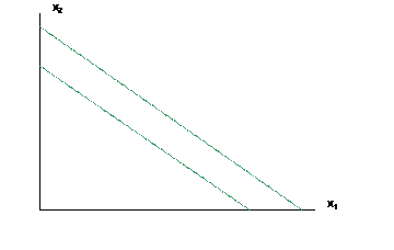
d. note effects of an income shift, Dm, a parallel shift of line;
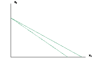
e. effect of price shifts, Dpi, where the new line is no longer parallel and budget rotates around one intercept (the one whose price didn't change). In picture below, a fall in the price of x1 means that more of x1 can be bought if the consumer devotes entire budget to it.
f. and the special case of an equal proportional change in m and all prices so there is no net change
|
3. Utility |
|
|
a. From Micro, recall that as long as a consumer's choices satisfy some basic requirements then the choices can be represented by a utility function
b. Define Marginal Utility, MU1, MU2 as MU1 = ΔU/Δx1 and MU2 = ΔU/Δx2 (For those with calculus knowledge, then MU1 is the derivative of the utility function with respect to the first argument, MU1 = and MU2 = . If you don't know calculus then ignore this note!)
c. MRS =
d. So draw indifference curves

|
4. Choice |
|
|
a. Given and a budget constraint that
b. we want to find the goods, x1 and x2, that solve: subject to .
c. Usually optimal point is at a tangency, where or or .
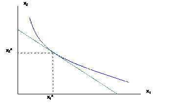
d. The last condition is "bang for the buck"
An example from Thomas Friedman's NYTimes column of Sept 15, 2006:
Since
the 1970’s oil shocks,
|
5. Effects of Change in Income |
|
|
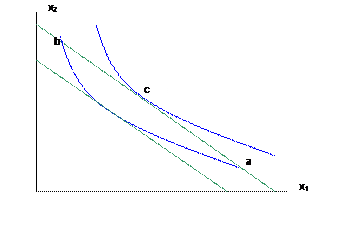
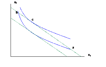
a. As income, m, rises the consumer could buy more of both; can choose any point that is between the intersections of the old indifference curve with the new budget (a and b in the figure below):
or
or
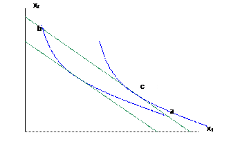
Clearly it is possible that, as income rises, an individual could choose to purchase more of both x1 and x2, or more of x1 and less of x2, or less of x1 and more of x2. It is perfectly reasonable that there are certain goods that people buy less of, as they get richer. Indeed most marketers of consumer goods offer a whole constellation of brands that aim to help people work "up the chain" as they get wealthier. What clothing brands are for poorer (often teen) consumers? For middle-income ones? For the rich?
b. We don't want to limit ourselves to only certain sorts of goods so we allow the consumer to have this range of choice. If people buy more of a particular good as they get richer, economists call this a normal good. Mathematically a normal good, xi, is one where . An inferior good, xj, is one where .
c. Graphically we can plot the income offer curve or income expansion path as showing the bundles of x1 and x2 that the consumer chooses at each level of income:
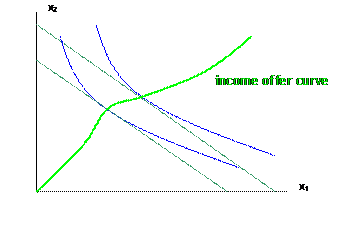
It is the locus of tangent points of the indifference curves and budget line. Of course it is different for every price combination.
d. We also can consider the Engel curve, which is a plot of the quantity of a good, xi, and the level of income, m (with the dependent variable on the horizontal axis, just to confuse you!).
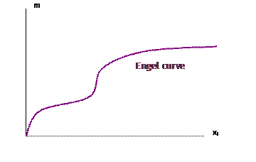
i. The Engel curve is not always upward-sloping, however. Slopes up only for normal goods.
ii. Inferior goods would have an Engel curve sloping downward. (It's also possible for some goods to be initially normal and then inferior. For instance calorie consumption: in poor societies the richer people are fatter because they can afford not to starve; in rich societies the richer people are more fit because they can afford to exercise and eat better.)
|
6. Effects of Change in Own Price |
|
|
a. From and , we now consider how the optimal choice of xi is influenced by changes in its price, pi.
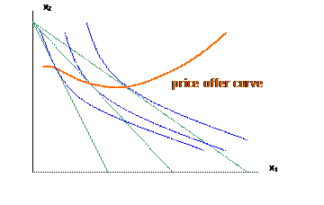
b. Now if we keep income constant but instead change p1, we can observe how the consumer's choice of bundles change. Linking these together gives us the price offer curve:
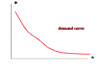
c. A plot of the price against the amount of the good chosen (again, putting the dependent on the horizontal axis) gives us the demand curve:
|
7. Examples |
|
|
We can get mathematical representations for these given functional forms for utility functions.
Basic common utility functions with easy solutions:
· Cobb-Douglas, for instance U = sqrt(X1,X2); a variant is U = ln(x1) + ln(x2) but you should be able to show that this is a monotonic transformation of the previous case
· quasi-linear U = sqrt(X1) + x2
· perfect substitutes U = ax1 + bx2
· perfect complements U = min(x1, x2)
Set budget = m, p1 = p and p2 = 1 (so p2 is numeraire, without loss of generality)
Cobb-Douglas case with so and .
Solve the bang-for-the-buck condition to find , , , , , . Put this into the budget constraint that , , . Then put this back into the result of the bang-for-the-buck, so . So from this we can sketch the Engel curve and demand curve for good x1: the Engel curve is a line from the origin (re-write, since the Engel curve puts m on the vertical axis, as ); the demand curve is a rectangular hyperbola (again, re-write with p on the left).
You should be able to solve the more general case, .
Quasi Linear, so , . Bang-for-buck gives . Solve for -- but only if there is enough money to buy this amount! The bang-for-the-buck shows that the consumer first has MU1/p > 1 at a low level of x1, but then this is satiated and the consumer spends any increase in income on x2. The budget constraint gives , so (as long as this is non-negative).
I will leave the perfect substitutes and perfect complements as an exercise, since we don't make much use of those in this course.
|
8. General Equilibrium: Edgeworth Boxes |
|
|
Up to now we have been looking at partial equilibrium solutions: taking some factors as exogenous, asking how demand and supply in a particular market would change. But of course demand and supply in any particular market depend on demand and supply in other markets, as the news regularly reminds us: the property price bubble led to unusually high demand for certain goods; high gasoline prices restrain consumer demand; there are always linkages. We want to build a model that can account for these, that is a general equilibrium (G.E.). Walras was one of the early economists to devote himself to this sort of theorizing, so these models are sometimes referred to as Walrasian general equilibrium.
We first look at an economy with 2 people trading 2 different goods. We assume that they are endowed with a certain amount of each good and then can trade to achieve their optimum level. So let's lay out the notation first. The people are A and B; the goods are 1 and 2; so that is the consumption, by person A, of good 1, is the consumption of good 2 by person B (the 2 superscript does not mean that x is squared). We denote the endowments of each good with .
So given prices, p1 and p2 set in the market, each consumer wants to maximize their utility given their budgets; so person A will
subject to
and B will
subject to , where as long as "more is better" the less-than-or-equal-to signs are equalities.
Changing prices will give incentives for the consumers to change their consumption choices – we sometimes explicitly show that the final consumption choices, depend on the prices by writing them as .
Each consumer might choose to consume either more or less than she is endowed with, so either demanding more than she has or supplying some of what she has. We define the "excess demand" function of each person, i=A,B, as:
and . So we could re-write each person's maximization problem as:
subject to .
How would we define equilibrium here? Certainly we need the condition that the same quantity that is bought is equal to the quantity supplied (supplied by the endowments of goods). These conditions, the global resource constraints, for each good are:
and .
One of the key considerations of this model is that consumers don't need to know the global resource constraints, just the price of a good, when making their choice. In the 2-person case the informational savings do not seem that big – consumer A only needs to know p1 and p2 rather than person B's choices of goods 1 and 2, but as the number of consumers increases, the efficiency of the price signals increases. Imagine if there were just 100 people trading the 2 goods – a consumer in a decentralized market economy needs only to know p1 and p2 rather than the 198 choices of 99 people of 2 goods!
However the details of price formation are left rather dangling. In the Walrasian case we assume that there is some agent that is the "auctioneer" who calls out prices, gets information from each agent about how much they would demand or supply at those prices, nets up the totals and then changes the prices as necessary. In the real world there is no such auctioneer – although maybe someday eBay will be!
What are the conditions that these prices need to fulfill? We can re-write the global resource constraint conditions, that and , by instead putting them in terms of net demands, so giving us the aggregate excess demands for each good as z1 and z2, where:
and
or, dropping the extra notation about dependence on prices as well as the summation notation, this is:
and .
So equilibrium is a set of prices that give both z1 = 0 and z2 = 0.
However those 2 equality conditions are actually redundant. The maximization constraints for each agent imply Walras' Law, that:
for all p1, p2 > 0.
This "Law" can be verified by substituting in the definitions of z1 and z2 as excess demands, then noting the budget constraint for each consumer, that .
So if we have k goods then the k prices, in order to be equilibrium values, must set (k – 1) aggregate excess demands to zero (and Walras' Law will take care of the last). The intuition of this result is that, given the way we have specified each consumer's problem, their choices of consumption depend entirely on relative prices, not the absolute levels. So the equilibrium values would not be changed if the consumers used different currencies, or if all prices were increased by a factor of 10, or if there were general inflation. In other words, these consumers have no money illusion.
Under what circumstances, or what restrictions on the preferences of the individuals, can we assert that an equilibrium must exist? Basically, if the functions z1 and z2 are continuous, then this will assure that there is a decentralized competitive market equilibrium. Continuity can be assured if all consumers have convex preferences (so that small changes in prices give small changes in their demands) or if there are many consumers (so that, in aggregate, even if a few consumers make large changes in demand in response to tiny changes in price, the total demand does not swing too far).
The Edgeworth Box diagrams provide an elegant visual explanation for the market processes (although it is difficult to diagram more than 2 people with 2 goods; unlike the functions above where adding more people or more goods is straightforward).
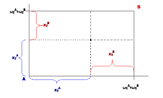
The Edgeworth Box puts a different set of axes starting at the point, , so that every single point in the diagram gives 4 pieces of information: the horizontal axis gives the consumption of good 1 by person A (the remainder is consumed by person B so it also shows since the total consumption must sum to the total endowment, ) and the vertical axis shows consumptions of good 2 by A and B.
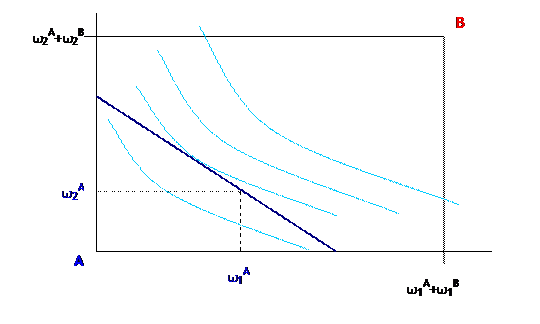
So the indifference curves and budget line of consumer A would look like this:
while the indifference curves and budget line of consumer B would be as below (turn the picture upside down if it doesn't look familiar):
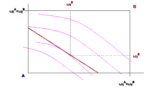
So the combination is:
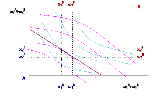
where the diagram now shows the initial endowments, ,
and the final equilibrium consumption, ![]() – whew! are there enough lines in that picture
yet?! The equilibrium market price is
how we get from the initial endowments to final consumption.
– whew! are there enough lines in that picture
yet?! The equilibrium market price is
how we get from the initial endowments to final consumption.