|
Basic Background Knowledge: Review of Economics for Economics students 2. Firms Economics of the Environment and Natural Resources/ Economics of Sustainability K Foster, CCNY, Spring 2012 |
|
|
One input was done in the basics especially for SUS students.
|
1. Multiple Inputs |
|
|
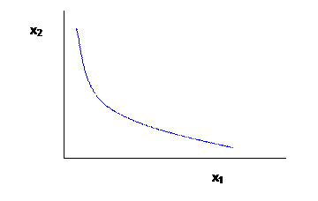
We graph the interaction of two inputs to make a particular amount of output by showing an "isoquant" – a very unlovely word! An isoquant connects together different amounts of inputs that give the same level of output. (Analogous to indifference curves.)
In a simple case, say we want to move a specified amount of dirt (dig a hole or fill in a hole or whatever). We could do it with a lot of people with basic tools, or gradually give some people more powerful tools and hire fewer people, all the way to having only one or two people running gigantic machines. There's no necessary reason that one or the other is better, the firm only cares about prices. If people can be hired cheaply then the firm will use more people; if machines are cheap then the firm will use machines.
We could imagine perfect complements or perfect substitutes in production or anything between. Typically the isoquants are assumed to be convex, for reasons similar to what was explained above in the one-input case.
As you can probably guess, we want to find an equation for the slope of the isoquant, which is called the Technical Rate of Substitution, or TRS. The TRS tells us how many of input 2 must be added, when one unit of input 1 is removed, to keep output constant. Again to figure out the TRS, imagine that we cut input 1 by units – how much would output be expected to fall? We would expect . But if we wanted to keep constant then we would need to balance this with an infusion of input 2, in amount of , just enough that . From this we see that .
Just as with the indifference curves, we expect that there should be a diminishing TRS as input 1 is increased. This comes about from the assumption that each input has diminishing marginal productivity: as input 1 increases and input 2 is cut, will fall and will rise so TRS will fall as input 2 rises.
The firm will minimize costs, subject to producing a given level of output, at the tangency of the isoquant and isocost, where the slopes are equal. Another way of thinking of this is to go back to the "bang-for-the-buck" concept. A firm with one more dollar to allocate to an input wants to make this dollar go farthest – which input choice would make more output? Note that this is not absolute productivity (a multi-million dollar machine might be more productive than a hammer, but it also costs a lot more) but productivity scaled by dollars. How much more output would be produced by spending one more dollar on input i? This is . If a dollar spent on input 1 makes more output than a dollar spent on input 2, then the firm should adjust its input mix to choose more of 1 and less of 2, and vice versa. This only stops when . (This should look very familiar!)
|
2. Algebraic Examples |
|
|
If production is Cobb-Douglas, then and (sometimes these are written and , which is easier, but I'll show it the hard way). Note the diminishing marginal products (graph MP1 as a function of x1). Use the bang-for-the-buck condition to find , , . Substitute this into the production function, that , , , or since y is known (it's the target output level), . This looks a bit fearsome but is actually just a linear function of y. Put this into the earlier relation from the bang-for-the-buck so . Put this into the cost function, that , so , . This shows constant returns to scale: as output doubles, so too does cost.
You should be able to solve this for a more general Cobb-Douglas form, , as well as the form, . (No shortcuts this time! Monotonic transformations change the production function!)
|
3. Costs in Short Run |
|
|
Marginal Cost is the change in cost per change in output, . Marginal cost is not generally constant but varies with output.
We define several other costs:
Average cost, AC, is the cost per unit of output, .
In the short run, some costs are fixed (F) and some are variable, .
Average variable cost, AVC, is the variable cost per unit of output, .
Average fixed cost, AFC, is , but since F does not change, this is just a rectangular hyperbola and doesn’t change much – so we rarely pay much attention to AFC. However we note that AC = AVC + AFC.
Also, from the definition of marginal cost and of fixed cost, we note that there is no need to define both marginal total cost and marginal variable cost – since fixed costs don’t change, marginal fixed costs are always zero so marginal total cost and marginal variable cost are always identical: .
These SR curves are typically graphed as:

Where we note that MC must intersect AC at the minimum point of AC; also MC must intersect AVC at the minimum point of AVC. To show this, note that by definition if MC>AC then AC must rise; if MC<AC then AC must fall. The minimum point of AC is where it turns from falling to rising, where it, for at least a short (infinitesimal) time it is neither rising nor falling so MC=AC. Same argument goes for AVC.
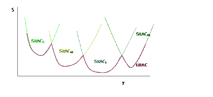
In the long run, there are no fixed costs, so long-run average costs (LRAC) are equal to long-run variable costs. LRMC are defined analogously to the short run.
LRAC can never be greater than the short-run AC curves – having more choices can never hurt profits!
In Long Run there are no fixed costs (can always choose zero output at zero cost). LR AC curve is envelope of SR AC curves – with a scalloped edge if there are discrete plant sizes but, as plant sizes become continuously variable, the LRAC becomes a smooth curve.
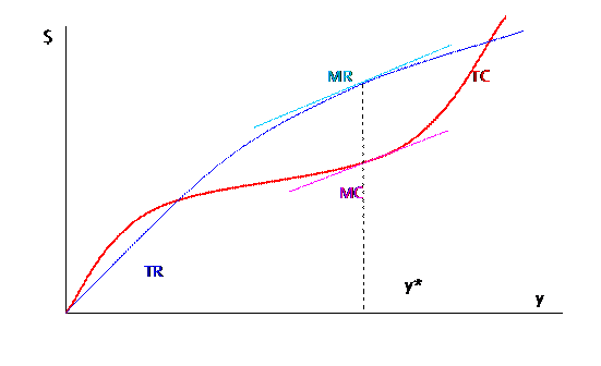
To maximize profit the firm will set . Consider this graph, where MR is allowed to vary as well as MC. To maximize profits, the firm wants to find where TR is farthest away from TC. The usual argument applies: making and selling one more unit of output raises revenue by MR; making one more unit of output raises costs by MC. If MR>MC then this was a good choice for the firm and it should raise output more. If MR<MC then this increased output was not a good choice and it should decrease output. It will stop this changing and reach equilibrium where MR=MC. In perfect competition where P=MR, this gives us the equilibrium condition P=MR=MC.
|
4. Profit Maximization in Short Run |
|
|
Assume that the firm faces MR = p, which is the amount by which revenue increases when output rises. Again, if MR>MC then the firm will produce more; if MR<MC then less.
So a firm with these cost curves (which we describe as canonical):
could face prices that lie in 3 separate regions: (A) either price intersects MC where MC is above AC; or (B) price intersects MC where MC is below AC but above AVC; or (C) price intersects MC where MC is below AVC.
Consider (A):
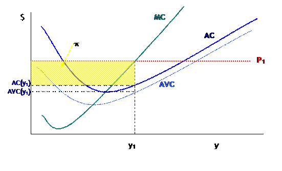
in this case, when price is at P1, the firm will choose y1 level of output to maximize profits. Profits are but can be more easily seen graphically as . So profits are drawn as the area of the rectangle with height and width , marked yellow in the graph. The decomposition of costs into Variable Costs and Fixed Costs can also be seen: VC are the area of the rectangle with height and width ; FC is the area of the rectangle with height and width .
With price at (B), where it intersects MC where MC is below AC but above AVC, we find:
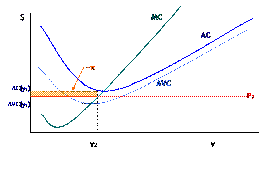
Again the firm chooses the point where , which is . Profit here is actually negative, since , the firm's average costs are greater than average revenue. So the question arises, is the firm really maximizing profit? Well, what else could the firm do? It could shut down completely, but in this case it would lose , which, in the diagram, is again the area of the rectangle with height and width -- and this rectangle is clearly bigger than the actual profit lost. Basically, since operating costs (AVC) are below the price, it makes sense to operate even if the firm doesn't cover all of its fixed costs. It covers some amount of its fixed costs and so reduces its losses. This is just another manifestation of the old rule: sometimes the best that we can do still isn't very good. The firm is maximizing profits but still losing money.
Only in the case of (C) would the firm actually shut down. Consider:
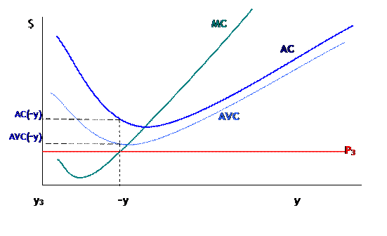
Now with price at , the firm could choose to continue producing where , at the point labeled (from computer programming, the tilde means "Logical Not"). But at this point, the losses to operating, totaling would be larger than the losses to just closing down and losing fixed costs, the rectangle of area . So the firm chooses whenever the price is less even than average variable costs.
This tripartite division has many real-life ramifications. This is why hotels and airlines are willing to give last-minute deals: a butt in an airplane seat paying even $20 is more than the extra cost for the jet fuel to haul that little bit more weight. They try and try to charge more, to cover their fixed costs, but when it comes right down to the end they know that their variable costs are low.
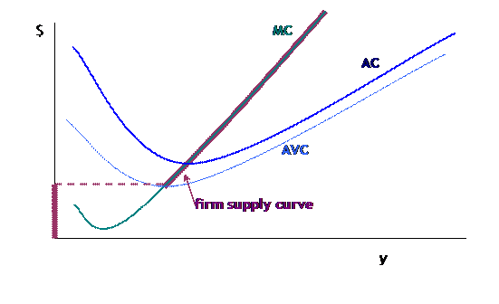
Firm Supply Curve
The firm's supply curve is then the locus of price and quantity choices, which is the firm's MC curve above AVC, then quantity jumps to zero if the price falls below this point. In the graph, this is:
|
5. Example |
|
|
Suppose costs are . What is the firm's optimal size? Find . Clearly fixed costs are F; then variable costs are so . . You can graph these – they're a bit different than sketched above, to keep the math under control. Optimal size is where MC=AC so , solve to find .
You can try some more examples, such as TC = 20 + 2y + y2 or TC = 100 + 4y + 4y2.
|
6. Hicks-Marshall rules of Derived Demand |
|
|
Pass-through of price changes depends on Hicks-Marshall rules of Derived Demand:
a. Demand for input is more elastic when
i. technical substitution is easy
ii. input cost share is high
iii. input is supplied elastically
iv. demand for output is elastic
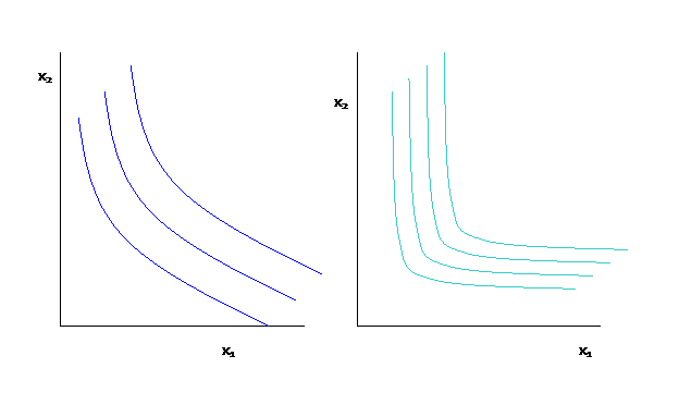
Take each one in turn. #1 means that isoquants are as on left not on the right,
#2, that cost share is high, means that there is a substantial pass-through of this particular input cost,
#3, that input is supplied elastically, means that if #1 is fulfilled (it is technologically feasible to get more or less of the input), it will not change the price of that input to buy more or less,
#4, that demand for the output is elastic means that changes in price have a significant change in demand for the output.