Lecture Notes 3

Economics of the Environment and Natural Resources/Economics of Sustainability

K Foster, CCNY, Spring 2012

Short Review of Production

1. Firms Choosing How to Produce

Assume that firms want to maximize profit, π, which is Revenue minus Cost. This is far from a perfect description of the world of course but it's a start.

Split the production decision into two parts: first, if a firm wants to make a particular quantity of output, what is the cheapest way to make it; second, how much output will a firm choose to make. This division allows us to focus on particular pieces first.

The first question to make a particular quantity of output, what is the cheapest way to make it? gives us the single essential number: the cost of that amount of output. The cost of this output is the only important item that the firm, when choosing amount of output to produce, needs to know. It does not need to know the quantities of inputs or relative costs. This split can also be thought of as reflecting a firm's organization: there is the corporate level that makes the decisions about how much product to make, if those output levels have a particular cost. Then these decisions are communicated to the plants that make the output, where each plant manager is told to make a particular amount of output, using the cheapest input mix possible. The plant manager doesn't need to know how a particular quantity of output was chosen; the corporate level doesn't need to know details of how that output is made, just the cost.

At this level we are not paying attention to questions of corporate structure. Given the decision structure from above, we might think of the plant managers as being a separate firm, outsourcing production. (A brand-name computer maker buys chips from a separate company; it doesn't need to know details of how the chips are made, indeed that might be a close-held secret. All it needs to know is the cost.) Our modern economy has many such firms providing corporate services, from high-level research down to the company cafeteria. The informational savings are immense: a firm doesn't need to know the details of how each input is made, it just needs to know how much they cost. If they want paper, they don't need to ask about how many trees grew for how long, they just need the cost per ream. (This is why central planning fails, since there are no prices and so no informational savings.)

We begin our analysis at the base, at the level of the plant, which is given an order for a particular quantity of output and must choose how to most cheaply make it. Again we divide the decision into two parts: first asking what is physically possible (what inputs can make the output) and then asking which combination is cheapest.

2. One Input

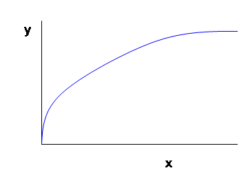
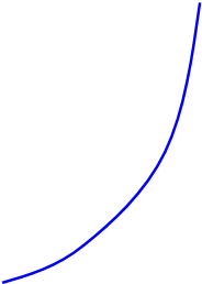
The simplest case is where one input makes one output, so we simply have . The marginal product of the input is how much additional output is made by adding more input, or , which is the slope of the graph. Assume that it is increasing, continuous and convex.

The assumption of being an increasing function (i.e. that ) is anodyne. Just as with utility, if output actually falls when inputs rise then you don't need an advanced degree to figure out that you should cut back. The interesting problem occurs when output could still be increased and you want to figure out if it is profitable.

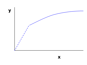
The assumptions of continuity and convexity don't seem as obvious. But they can be solved if we think of the firm's problem over a slightly longer period. Suppose that a firm's underlying physical process of production is discontinuous: it takes at least 100 units of input in a day to make 100 output units, but less than 100 of the input just won't even start up the machine. Is the firm's production function to be considered discontinuous? Well what if the firm got orders for 50 units of output per day what would it do? Clearly it could just run the machine every other day, and average 50 units of output with 50 units of input per day. If orders run at 80 per day then the machine is run on 4 out of 5 days, and so forth. Of course this assumes that the output is storable and that the time over which we are speaking is relatively short (more on this later). But the assumption is not too bad.

The convexity assumption comes by the same assumption. If the firm can make 100 output with 100 input then it could make at least half as much output with half the input. (On the graph, any chord drawn between 2 points will lie on or beneath the production function.) If there were non-convexities in the underlying physical process then, again, production could be structured to avoid these.

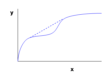
The convexity assumption is also why we often talk about a "Law" of Diminishing Marginal Product. It is reasonable to assume that the Marginal Product, , is diminishing (or at least not increasing) because if it were increasing then, as in the graph above, the firm would want to figure out ways to exploit this.

Clearly, assuming just one input to the production function is restrictive. I can't think of too many things that are produced in that way (except for the world's oldest profession). We want to consider multiple inputs.

3. More than One Input

We commonly limit ourselves to two inputs because that allows easy graphing and still gets to most of the complexities. But you should be able to see how the number of inputs could be increased.

Now describe the production plant with a production function where inputs are transformed into outputs by way of a production function: . We could imagine a wide variety of production functions but we assume that it has some basic properties. Note that, whereas in the consumer problem, we were reluctant to make restrictions directly to the utility function and instead discussed assumptions about the underlying preferences, that was because utility was un-measurable and only a convenient descriptive device. Production is more easily measured as long as there is some physical output: tons of steel or pairs of sneakers or casks of beer. So we make assumptions directly about the production function.

We again assume that the production function is increasing (so more inputs lead to more output), continuous, and convex (or something like convex). Now define each input's Marginal Product: , where we use the function notation to remind ourselves that the MP for each input is likely to be different, for different levels of each input. This is important there are likely to be complementarities in production. The Marginal Product of one input is likely to depend on the levels of other inputs as well. (For example we often hear statistics that workers in third-world countries are not as productive as US workers this doesn't mean they're any worse, just that they have different levels of other inputs.)

Again we assume diminishing marginal products, that falls as input 1 rises (holding constant input 2) and vice versa. This "holding constant" part is particularly important since, while in the long run we might be able to increase output by increasing both inputs, in the short run one input or the other is usually less flexible. Consider the typical office worker nowadays, who usually gets one computer. If a company hires more people without buying more computers, then the productivity of the new people (whatever their talent!) will be limited as they have to jostle for computer time. Similarly if the company got new computers without hiring new people a few people might get multiple computers on their desks, and some might be more productive with those new computers, but not very much.

This is distinct from returns to scale, which asks what happens to output if all of the inputs are increased. Hiring people without getting more computers might not raise output much; getting computers without hiring more people might not raise output much; but hiring more workers and giving each a computer might still raise output. Diminishing Marginal Products for each input alone does not imply diminishing returns to scale.

To more formally define returns to scale, suppose a firm doubled its inputs, and ask what would happen to outputs? If output doubled exactly then a firm would have constant returns to scale (CRS). If output increased by more than double then the firm has increasing returns to scale (IRS). If output increased by less than double then there are decreasing returns to scale (DRS). To put this a bit more abstractly, we compare the output from doubling the inputs, , with twice the original output, . If then production is CRS; if then IRS; if then DRS. Or, more generally, for any scale factor , if then production is CRS; if then IRS; if then DRS.

Short Run vs Long Run

Often one input is more flexible than the other. This means that our analysis should distinguish between the short run (when one input is fixed) and the long run (when both inputs are flexible). Often we assume that labor is flexible and capital (the machines) are fixed since building, say, a new assembly line takes time. But other firms might have different rankings universities have tenured faculty, many of whom have been there longer than some of the buildings on campus!

4. Profit Maximization

A firm's profits are revenues minus costs, so a firm selling n different output goods, each for price p_i, and using m different inputs, each with cost w_j, would have profit .

First note that the costs must all be put into the same units dollars per time unit. Which raises the question, if a firm buys, say, a truck that is expected to last for 5 years, how is this cost compared against the daily wage of the person driving it? To answer this we suppose that another company were set up that just rented out trucks: it goes to the bank, gets a loan to buy the truck, and then charges enough per day to pay off the loan per day. We consider that, even if a company doesn't actually rent the truck but actually buys it, that it could have rented the truck. So the rental rate is the correct cost of that capital good. In the real world more and more companies are separating their daily operations from their loan portfolio and renting equipment. If you work at an office, you know that most photocopiers are rented. Airlines rarely own their own jets, they rent them. Offices are usually rented space. (Employees are rented, too!)

The companies have figured out that correctly measuring costs allows them to make better decisions. Capital goods which are owned and given away internally as if they had zero cost are not efficiently used.

Economists also measure costs differently from the way that accountants do regarding payments to shareholders/owners. If a public company has an IPO and sells its shares for $100 each, then those shareholders expect something in return. They expect that the dividends (and/or capital gains) will return them as much or more money as if they had invested their $100 in some other venture. So the company had better return $8 per year if the investors could have gotten 8% returns. An accountant would count this $8 per share as a "profit" but economists see that as a cost to be paid to shareholders for the use of their money (their capital). If the firm were to return just $6 then the shareholders would be angry and the firm would be in trouble; if the firm returns $12 then the shareholders are delighted.

So economists often talk about "zero profits" being a general case, which makes people wonder how much economists know about the real world since any business newspaper daily reports companies making "profits". But we're just counting different things. If the regular return to capital is 8% then, if the firm makes $8 that the accountants call profit, we call it a cost and report that the firm made zero economic profit.

5. Profit Maximization with One Input

This means

subject to . Hiring one more unit of input will raise the firm’s cost by ; this one additional unit of input will raise output by and so revenues will rise (assuming no market power) by , which is the value of the marginal product. If then the firm should hire more inputs; if then the firm should hire fewer inputs; so in equilibrium .

Note that, if one input is fixed, then even the two-input model becomes, in the short run, just this problem of profit maximization with one input.

6. Profit Maximization with Multiple Inputs

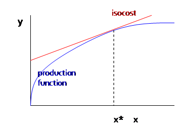
Now the firm is to subject to . Again the same logic applies. Hiring one more unit of input one will raise the firm’s costs by and raise revenues by so in equilibrium and . Also these imply that our usual bang-for-the-buck marginal conditions apply, that which is the tangent condition that the slope of the isocost equals the slope of the isoquant at optimum. This condition gives the long-run profit maximizing combination of inputs to be used, which allows us to derive the long-run cost function.

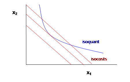
To make a particular amount of output, in the long run the firm minimizes cost by choosing to produce with the inputs set at the tangency.

Cost Minimization/Profit Maximization

The firm’s problem to maximize profits generates a dual (sometimes easier) problem, which is how to minimize costs subject to a constraint of making a particular amount of output. (The constraint is important, though -- if the firm wanted to minimize costs without that constraint, clearly setting y=0 would be best!)

If the firm wanted only to maximize revenue (or if the input were costless) then the firm would subject to . A "costless" input sounds crazy but remember that Mankiw says, "rational people make decisions on the margin." Zero marginal cost is not that unusual: it's the usual condition for media companies they pay a big fixed cost (to record a song or make a movie or TV show), but then their marginal costs are about zero: one more iTunes download does not cost them much!

7. Marginal Revenue

To figure out this problem of zero marginal cost but changing revenue, we just need another definition. Marginal Revenue, MR, is the change in revenue per change in output, . If price is a function of the level of output (e.g. the firm has monopoly power) then MR can be a complex function. If the firm operates in a competitive market then the price is outside its control, so the increase in revenue from selling one more unit of output is the price, p.

But many firms have monopoly power. Consider a fashion label selling handbags. They want to sell more because that means more revenue. But they also know that scarcity has value: some designers sell in only a few select boutiques and can charge very high prices; other designers sell bulk quantities in department stores and cannot charge high prices. This is a very general problem.

A firm that wanted just to maximize revenue would expand production as long as MR>0 and only stop when MR=0, when producing more output would no longer raise its Revenue.

Most firms, however, do not simply care about maximizing revenue; they want to maximize profits. (Particular parts of firms, however, might want to maximize revenue: for instance, most sales people are paid commissions on the sales they generate not necessarily the profits. Countrywide got paid per mortgage regardless of quality.)

A firm that wants to maximize profits will also have to take account of Marginal Cost. It is also convenient to figure other cost definitions.

In a perfectly competitive environment the firm's demand curve is a horizontal line the market price for this homogenous commodity. The firm can sell as much quantity as it can produce at that price. Lowering the price will not increase the amount sold; raising the price will stop all sales. This is an extreme assumption but, as you think about it, not completely unrealistic. One of the important points of any business plan for a new company is 'the competition' what other firms sell and at what price. If my firm offers the same product then I can't charge a higher price. Of course my firm might charge a higher price and offer a better product, but this means that I'm selling a different output.

The business press sometimes discusses the "commodification" of different markets: for example at one point, when computers were new, the chips were quite different and there were many different prices; now that chips are standardized there is much less variability in price. Financial markets are commodity markets: nobody offers a "20% sale" on stocks or bonds! Markets are organized in order to standardize and "commoditize" certain products: e.g. the CBOT offers corn futures to deliver "5000 bushels of No. 2 yellow corn"; or "100 troy ounces of refined gold not less than .995 fineness cast as one bar or 3 one-kilogram bars"; the NYMEX trades gasoline "reformulated gasoline blendstock for oxygen blending (RBOB) futures contract trade in units of 42,000 gallons (1,000 barrels)" for delivery in New York.

This is not to say that the market demand curve is flat, just that the curve for the particular firm is flat. Another way of thinking of it is that the firm is such a tiny player in the whole market that it sees just a tiny piece of it, which is essentially flat. But even if there are a limited number of companies then a firm might still face a flat demand curve for its product based on the other's price. A final example: whatever I sell nowadays, I have to know what Amazon or eBay charges for it most all of my customers will!

Production Externalities

In the simplest case, we can examine a firm making a single private (rival and excludable) output and incidentally a single public (nonrival and nonexcludable) output (for now, we assume that this public good is disliked). An easy example could be a power plant which makes electricity and pollution. (Actually a variety of sorts of pollution, which affect different groups of people: carbon, mercury, NOX, and sulphur dioxide are the main ones.)

In this case the production can be shown as being like a production possibility frontier but with the pollution increasing along with the output, something like:

The firm can choose any combination of electicity & pollution within the light blue area. Clearly, however, the firm would be foolish to choose a point inside the area; the points at the dark blue line are efficient. These are the production possibility frontier. They are efficient because there is no way to increase the output of electricity without also increasing the output of pollution (this would not be true for points in the interior).

At any point along the frontier of production possibilities, we can define the marginal rate of transformation as the change in output of pollution per change in output of electricity the slope of the line. With the notation of e for pollution emissions and y for the output of the firm, the marginal rate of transformation, MRT, here is , where is the function linking the amount of emissions generated as determined by the amount of output produced. We can think of electricity generation as transforming some amount of a public good (in this case clean, unpolluted air) into a private good (electricity).

This interpretation of the choice along the production possibility frontier as representing a choice of marginal rate of transformation allows us to compare firms and make statements about the relative efficiency.

Suppose there are two firms which, for some reason or another, have different emissions per unit of output. Graphically this would be represented as:

If they each produced the same amount of emissions, they would of course be able to generate different output levels, but their marginal rates of transformation would also be different.

Clearly the marginal rate of transformation of firm 2 is lower than the marginal rate of transformation of firm 1. This means that when firm 2 generates one more unit of output, it creates fewer emissions than firm 1 does. This means that, if firm 2 were to make one more unit of output while firm 1 made one unit less keeping the total output of the two firms at the same level, the increase in emissions from the second firm would be (in absolute value) less than the decrease in emissions from the first firm. So total emissions would be smaller even though the output was kept constant.

Consider a simple numerical example, where but . This is plotted as:

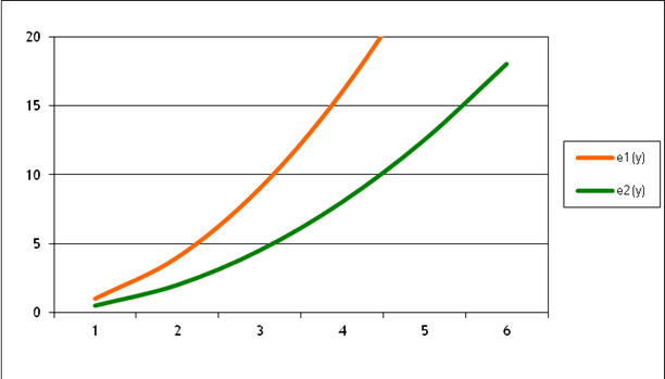
If emissions of each firm are 16, then firm 1 is producing 4 units of electricity while firm 2 is producing 5.66 units of electricity. If firm 2 produced one more unit of electricity its emissions would rise to 22.16, an increase of 6.16. If firm 1 produced one less unit of electricity its emissions would fall to 9, a decrease of 7. So if, instead of both firms producing 16 units of emissions, firm 1 produced less and firm 2 produced more, the overall production of electricity could remain constant while emissions fall.

We can continue this trade-off as long as the marginal rates of transformation are unequal. It is only when the marginal rates of transformation are equal that there will be a total efficient way of getting the most output with the least amount of harmful emissions. With a bit more math, we can find the point where the MRTs for each firm will be equal.

When we get to policy (next), we return to this idea: at the most efficient point, the marginal rates of transformation will be equal which will not necessarily be the point where emissions are equal.

Multiple Inputs

It is rarely quite appropriate to consider an output to be perfectly free, since there are usually at least technological considerations. So we can return to our usual marginal conditions, modified for the firm. Consider a firm which has multiple inputs available for making the output, each of which is useful and productive. Each input has a cost (or wage, if we extrapolate from the case of hiring workers) denoted w_i.

We typically assume that, holding all of the other inputs constant, increases to just one input will have a steadily-decreasing effect on increasing output. Graphically, this says that for each input, x_i, i=1, 2, … N, output, y, increases as:

So, just as with the consumer's diminishing marginal utility, the firm faces diminishing marginal productivity. Just as with the consumer, we define the production function as and the marginal product of each input as the partial derivative, .

Also as noted previously, the fact that each individual marginal product is diminishing does not mean that production overall has diminishing returns to scale where 'scale' refers to a case where all of the relevant inputs are increased. As a simple example, most offices generally operate with each employee getting a computer. Buying more computers without hiring more people might increase output, but at a diminishing rate; the same would hold true for hiring more people without getting more computers. But getting more of both could allow the business to expand.

The firm will maximize profits by choosing inputs such that (in the long run), the ratios of , marginal productivity per cost of each input, is equal. The explanation should, by now, be typical: if spending $1 more on input i increased output by more than spending $1 more on input j, then the firm should decrease spending on input i while increasing spending on input j. This will not only allow the firm to make more output more cheaply but also tend to bring down the marginal productivity of input j while increasing the marginal productivity of input i, so that in equilibrium we have .

If one input has a price which is increased (say, by some environmental regulation) then this input will be used less. This is the substitution effect (see from marginal condition).

There is also a Scale Effect. As the cost of production rises, the quantity of output demanded will fall, so fewer of all types of input will be demanded.

Also, if that input is non-excludable like polluted air or water, then other industries could see their costs fall, so input used more a different substitution effect. Also a different scale effect.

Hicks-Marshall rules of Derived Demand:

Demand for input is more elastic when

1. technical substitution is easy

2. input cost share is high

3. input substitutes are supplied elastically

4. demand for output is elastic

So putting the Scale effects and Derived Demand effects all together gets complicated. What is the impact of pollution restrictions on a firm, hindering its use of a particular dirty input? Clearly this adds to costs of the dirty input, but the impact of this cost change could be small or large depending on application of the Hicks-Marshall rules. Then what is the impact on other inputs (usually labor, i.e. jobs)? If the cleaned-up input is more labor intensive then this could mean a net rise in jobs; oppositely if the cleaned input is more capital intensive. If the cleaned input is more labor intensive, but the rise in cost greatly diminishes the demand for the product, then net jobs could fall if industry output falls. If the avoided pollution makes other factors more productive, then there could be further effects.

Might, for example, want to know the impact of a carbon tax on power plants. Here the share of inputs in total cost is clearly substantial; demand for output is inelastic that's easy. Technical substitution is happening in the long term (few new coal plants, many more natural gas plants that are dramatically cleaner) but in the short term is limited. Input substitution is complicated in long/short run: natural gas production from domestic sites is increasing while facilities for imports are limited; oil is not much better; nuclear plants are tough to build; new hydro or geothermal is limited; other power sources are available but with limits (e.g. uranium production, solar panels now often imported, biomass facilities, etc.). Natural gas shows the inter-relationship of #1 and #3 in Hicks-Marshall rules: new gas turbines are relatively easy to install but if there is a rush of new construction then natural gas prices (which have recently moderated) will rise again and the cost advantage of natural gas over coal would erode.

Supplementary Material for ECO students

Cobb Douglas Example

Consider a numerical example of a firm with a very simple Cobb-Douglas production function, so so the marginal products are (the last equation comes from a convenient simplification; it's a bit of a trick that's not obvious the first time you see it but you should be able to verify that it is, indeed, correct) and . The firm's cost is So put these expressions for the marginal products into the firm's marginal conditions that so so or . Put this into the production function to solve for so and -- these are the input demand functions, giving the firm's demand for each input as a function of both its output level and the relative price of the input. Put these into the cost function to find that the long-run cost is .

The long-run average cost is thus which sets the price in the market.

This allows us to easily see the scale and substitution effects. If the cost of an input, say w₁, rises, then this will mean that directly less of that input is used since ; this is the substitution effect. However it also raises the firm's average costs, in the long run so the amount sold must decrease. The size of this decrease in output depends on demand elasticity: if the output is elastically demanded then the price rise will produce a sizeable downward shift in quantity demanded.

Costs

The cost function is . It is determined, in the long run, by the wages of each input and by the level of output chosen. In the short run it is also determined by the amount of the fixed factor.

Marginal Cost is the change in cost per change in output, . Marginal cost is not generally constant but is commonly considered to vary with output.

We define several other costs:

Average cost, AC, is the cost per unit of output, . In the short run, some costs are fixed (F) and some are variable ( .

Average variable cost, AVC, is the variable cost per unit of output, .

Average fixed cost, AFC, is , but since F does not change, this is just a rectangular hyperbola and doesn’t change much so we rarely pay much attention to AFC. However we note that AC = AVC + AFC.

Also, from the definition of marginal cost and of fixed cost, we note that there is no need to define both marginal total cost and marginal variable cost since fixed costs don’t change, marginal fixed costs are always zero so marginal total cost and marginal variable cost are always identical: .

These SR curves are typically graphed as:

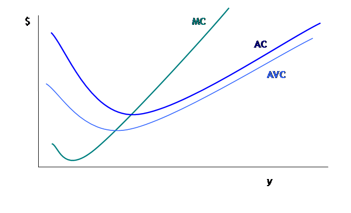
Where we note that MC must intersect AC at the minimum point of AC; also MC must intersect AVC at the minimum point of AVC. To show this, note that by definition if MC>AC then AC must rise; if MC<AC then AC must fall. The minimum point of AC is where it turns from falling to rising, where it, for at least a short (infinitesimal) time it is neither rising nor falling so MC=AC. Same argument goes for AVC.

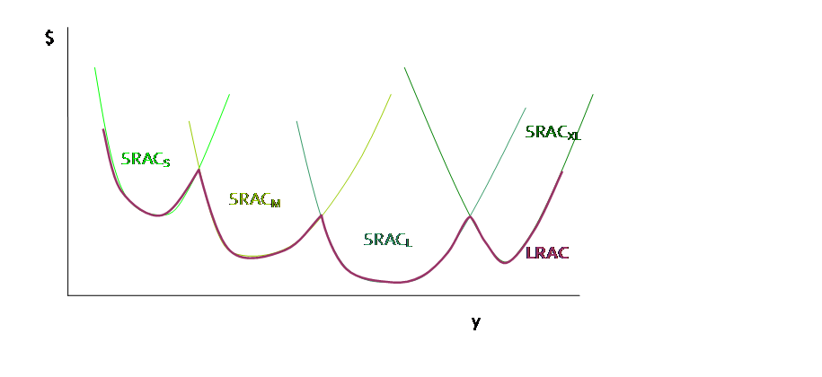
In the long run, there are no fixed costs, so long-run average costs (LRAC) are equal to long-run variable costs. LRMC are defined analogously to the short run.

LRAC can never be greater than the short-run AC curves having more choices can never hurt profits!

In Long Run there are no fixed costs (can always choose zero output at zero cost). LR AC curve is envelope of SR AC curves with a scalloped edge if there are discrete plant sizes but, as plant sizes become continuously variable, the LRAC becomes a smooth curve.

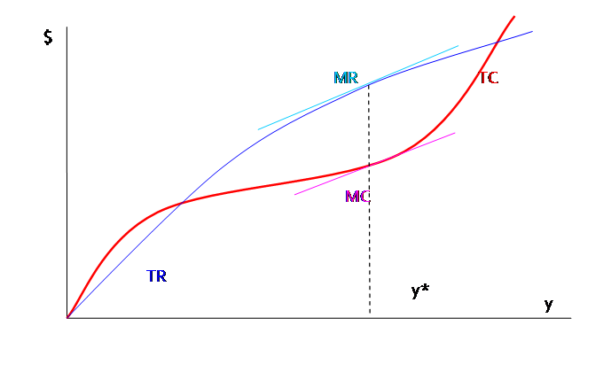
To maximize profit the firm will set . Consider this graph, where MR is allowed to vary as well as MC. To maximize profits, the firm wants to find where TR is farthest away from TC. The usual argument applies: making and selling one more unit of output raises revenue by MR; making one more unit of output raises costs by MC. If MR>MC then this was a good choice for the firm and it should raise output more. If MR<MC then this increased output was not a good choice and it should decrease output. It will stop this changing and reach equilibrium where MR=MC. In perfect competition where P=MR, this gives us the equilibrium condition P=MR=MC.

What is the firm's demand curve? In a perfectly competitive environment the firm's demand curve is a horizontal line the market price for this homogenous commodity. The firm can sell as much quantity as it can produce at that price. Lowering the price will not increase the amount sold; raising the price will stop all sales. This is an extreme assumption but, as you think about it, not completely unrealistic. One of the important points of any business plan for a new company is 'the competition' what other firms sell and at what price. If my firm offers the same product then I can't charge a higher price. Of course my firm might charge a higher price and offer a better product, but this means that I'm selling a different output. Sometimes I take a cab after class: whether I take a yellow cab with a meter or a black cab without, the price is the same (even though, for the latter case, it is negotiated at the end of the ride).

Profit Maximization in the Short Run

In the short run the firm must account separately for fixed costs. The profit maximization becomes: . Note that variable costs, , are a function of the level of output but "Fixed Costs are fixed." Fixed Costs don't change depending on the level of output, they're fixed. So the lowest level of profits that the firm could make are if output is set to zero (revenue and variable cost both become zero in that case). Beyond this, however, the usual rules apply. Recall that the marginal variable cost is exactly equal to marginal total cost. MC is how much cost increases when output increases. MR (which we assume to be in this case, for simplicity) is the amount by which revenue increases when output rises. Again, if MR>MC then the firm will produce more; if MR<MC then less.

So a firm with these cost curves (which we describe as canonical):

could face prices that lie in 3 separate regions: (A) either price intersects MC where MC is above AC; or (B) price intersects MC where MC is below AC but above AVC; or (C) price intersects MC where MC is below AVC.

Consider (A):

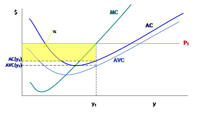
in this case, when price is at P₁, the firm will choose y₁ level of output to maximize profits. Profits are but can be more easily seen graphically as . So profits are drawn as the area of the rectangle with height and width , marked yellow in the graph. The decomposition of costs into Variable Costs and Fixed Costs can also be seen: VC are the area of the rectangle with height and width ; FC is the area of the rectangle with height and width .

With price at (B), where it intersects MC where MC is below AC but above AVC, we find:

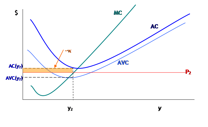
Again the firm chooses the point where , which is . Profit here is actually negative, since , the firm's average costs are greater than average revenue. So the question arises, is the firm really maximizing profit? Well, what else could the firm do? It could shut down completely, but in this case it would lose , which, in the diagram, is again the area of the rectangle with height and width -- and this rectangle is clearly bigger than the actual profit lost. Basically, since operating costs (AVC) are below the price, it makes sense to operate even if the firm doesn't cover all of its fixed costs. It covers some amount of its fixed costs and so reduces its losses. This is just another manifestation of the old rule: sometimes the best that we can do still isn't very good. The firm is maximizing profits but still losing money.

Only in the case of (C) would the firm actually shut down. Consider:

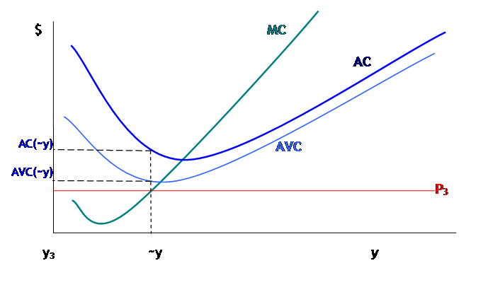
Now with price at , the firm could choose to continue producing where , at the point labeled (from computer programming, the tilde means "Logical Not"). But at this point, the losses to operating, totaling would be larger than the losses to just closing down and losing fixed costs, the rectangle of area . So the firm chooses whenever the price is less even than average variable costs.

This tripartite division has many real-life ramifications. This is why hotels and airlines are willing to give last-minute deals: a butt in an airplane seat paying even $20 is more than the extra cost for the jet fuel to haul that little bit more weight. They try and try to charge more, to cover their fixed costs, but when it comes right down to the end they know that their variable costs are low.

Another ramification is seen in the current housing bust. Driving through certain neighborhoods, there are still houses being constructed why? Clearly the answer is that, since the builder has bought the land (usually the most expensive part), that FC is lost now. If a house sits half-built then the construction company loses all the costs put into it so far. But even if completing the building takes more expense, it might still be worthwhile the builders will lose money, but not as much as if they walked away.

Firm Supply Curve

The firm's supply curve is then the locus of price and quantity choices, which is the firm's MC curve above AVC, then quantity jumps to zero if the price falls below this point. In the graph, this is:

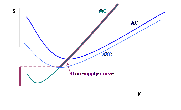
Examples of tax affecting either FC or MC depending whether it is per production plant or per unit of output. If pollution is per output but tax/regulation is per plant, this could have mixed effects.