This class aims to teach at least three different things – which are interrelated enough to make it sensible enough to jam into one class, but different enough to make it all complicated. These are:

1. Basic economics of sustainability and environment,

2. Basic business principles as applied to environmental enterprises.

3. Basic development concepts to understand the problem of global climate change,

The current version of these notes tries to cover part 1. Parts 2 and 3 will be later (??).

These notes are based on a number of different texts including Principles texts by Frank and Bernanke and by Mankiw, Intermediate text by Varian, finance text by Hull, environmental texts by Anderson, by Kolstad, and by Hanley, Shogren and White.

Basics

Although there are hard-core environmentalists who dispute it, believe that markets are the best way ever discovered by human ingenuity to efficiently allocate scarce resources and to ensure that resources are most effectively used. This is true for most resources but not all.

It is not true for all resources; this does not mean that no government intervention is ever justified. One of the objectives of this course is to figure out what institutional arrangements and structures allow markets to work, and which ones need to be improved. Where should government policy step in?

But a typical firm is run by managers who have a sharp incentive to cut costs: to limit the use of expensive inputs and to cut expenditures which do not directly impact customer satisfaction. Most consumers are looking for ways to cut their expenditures on items that do not bring adequate satisfaction.

So to begin, we will review basic economic theory about the allocation of scarce resources. In a perfect economy people don't need to understand all the implications of their consumption on different resources; they only need to know the price. The price is the sole sufficient indicator of scarcity. So much energy is expended by modern consumers trying to balance off different criteria, even for simple choices like a lightbulb. An incandescent bulb uses 'too much' energy relative to a fluorescent, but fluorescent bulbs usually contain mercury (hazardous disposal), other types of bulb might consume particular resources (rare earth metals) in being made. How ought consumers to trade off greater electricity usage versus mercury contamination? A consumer can be left swamped with information, trying to compare the incommensurable! But in a perfect economy consumers only need to look at the price. Clearly we don't live in a perfect economy.

But many resources are already included in the price of even the most quotidian consumption item. When we choose to buy an apple we needn't worry about whether the farmer has sufficient land or uses the proper fertilizer, or if the wholesaler has a good enough inventory-control system, or if the retailer uses scarce real estate optimally. We just choose whether or not to buy it. It's only when we try to trade off between organic apples or locally-grown apples or fair-trade apples or whatever – that's difficult, because there's no single scoring system.

In a system of optimal economic competition, the price reveals relative scarcity. If supply is low relative to demand then the price will be high; if supply is great relative to demand then the price is low. Early economists often wrote about the apparent incongruity that water, necessary for life, was available for free while diamonds, not necessary for anything, were expensive. Why this apparent paradox? Because of their relative scarcity. (And thus marginal utility, but that's for later.)

Over a longer time period, firms will direct their Research & Development (R&D) budgets towards economizing on items which are most scarce (i.e. have high prices) – again, just because it's profitable for them to do so.

These market processes are the basis for extraordinary wealth. For much of human history a person needed to work all year just to get enough calories to fend off starvation. Nowadays the developed world worries most about obesity.

Markets are extraordinarily powerful. Recall that many countries experimented with central planning (called Communism) and that was a disaster. The best efforts by very smart people (motivated, at times, by fear for their lives) were not enough to supply even a fraction of the goods that could be provided by a market economy. Wise policy will use markets wherever possible. However markets are neither all-powerful nor omniscient. There will be cases where the simple assumptions underlying the Welfare Theorems are no longer valid, particularly where there are substantial amounts of goods with imperfect property rights (with externalities) and/or substantial transactions costs. Bob Solow, the Nobel-prize-winning economist, refers to the free-marketeers who see the doughnut while the interventionists see the hole (Solow 1974 AER).

(e.g. Brad Delong delong.typepad.com/sdj/2010/12/what-do-econ-1-students-need-to-remember-second-most-from-the-course.html)

Define Economics

"Economics is the study of choice in a world of scarcity" (from intro text by Frank & Bernanke – yes, that Bernanke, who's just stepped down as Fed Chair)

Some resources, which were once thought to be inexhaustible, are now known to be scarce; e.g. atmosphere (CO₂ levels), clean air, fish in the sea
Scarcity: No Free Lunch (TANSTAAFL) – more of one thing means less of something else. This applies to buying groceries (more apples & fewer bananas) or choosing between car emissions & safety (lighter cars mean better MPG & less emissions but also less safe in accident).
Choice: people are free agents who take actions based on their own information and desires – which do not necessarily match those of policymakers. Usually assume people are rational.
Rational people think on the margins (Mankiw's intro text)
Cost-Benefit Principle: it is rational to take action if and only if the extra benefits are as big as, or bigger than, the extra costs

Economic Surplus = Extra Benefit – Extra Cost. So Cost-Benefit Principle can be restated as "Do actions with nonnegative Economic Surplus".
Opportunity Cost: The Extra Cost is the value of next-best alternative that must be given up to do something so Cost-Benefit means take an action only if it has nonnegative Economic Surplus; only if the extra Benefit exceeds the Opportunity Cost

If prices reflect true scarcity of all goods then people take proper account, not because of any moral feeling but to maximize profit. This goes back to Adam Smith's propositions and observations.
Environmental Economics is generally concerned with choices where the benefits and costs are shared even though the decision-making isn't necessarily

Here's a nice overview of Environmental Economics

Commodities and Goods/Services

· People buy and sell a multitude of different goods and services, many of them extremely specialized.

· Commodities are generalized goods, items that have been laboriously standardized in order to make them comparable.

· Commodities are created by people in particular situations (commoditization) – for example, the cafeteria buys apples as commodities by the thousand but then these same apples are chosen as individual goods (look for the ripest and least bruised fruit on display).

· Example, WTI Light Sweet Crude Oil (http://www.cmegroup.com/trading/energy/crude-oil/light-sweet-crude.html) is traded in units of 1000 barrels (each barrel is 42 gallons), delivered in Cushing Texas, where "light" and "sweet" are carefully defined physical qualities. Many lawyers worked to write up the documents that define this commodity and specify how variations are recompensed. Some details are in Chapter 200 (!) of the basic NYMEX rulebook http://www.cmegroup.com/rulebook/NYMEX/2/200.pdf. Oil companies work hard to ensure that a particular quantity of oil meets these standards.

· An exchange might create a new commodity that doesn't exist, such as "Crack Spread," the difference of crude prices and the value of the refined products.

Basics of Supply and Demand Curves

· Demand Curve:

o For each person: shows the extra benefit gained from consuming one more unit

o by Cost-Benefit Principle, if the extra benefit from consuming one more unit is greater than the price, then consume; if not then don't

o so Individual Demand Curve shows how many are purchased at any given price

o Individual Demand Curves are combined to get a market demand curve of how many would be purchased by all the people in the market at a given price (horizontal sum)

o Depend on other factors than price (which shift the demand curve).

· Supply Curve: opportunity cost of producing certain quantity of output.

o If no fixed costs and no barriers to entry then firms produce at marginal cost

o Depend on other factors than price (which shift the supply curve).

· Behavior of Markets: markets are a wonderful institution; we analyze with some assumptions

o Depend on composition of good

o Depend on supply characteristics (how many firms, if there are fixed costs or other barriers to entry, rules & regulations and social norms

o property rights are completely known, specified & enforceable

o all property rights are exclusive (no externalities)

o property rights are transferable

o items for sale have substitutes

o Commodities closely approximate these assumptions; other markets might be very far off (e.g. labor)

o What happens if demand is greater than supply? Vice versa?

· Equilibrium: price and quantity that have no tendency for change

· Some Common Mistakes

o Ignore Opportunity Costs

o Fail to Ignore Sunk Costs (since they're no longer on the margin)

o Fail to understand Average/Marginal Distinction

Jodie Beggs "Economists Do It With Models" on demand curves (follow youtube links for next lectures on supply; also Chapters 4, 5, 6 and 7 here, http://www.economistsdoitwithmodels.com/economics-classroom/)

Analyzing Supply and Demand Curves

· Consumer Surplus (CS)

You've surely had the experience: you go to a store to buy a particular item, ready to spend a certain amount of money. But surprise! You find it's on sale and you pay less than you expected. You've gotten Consumer Surplus. This did not come from the benevolence of the retailer (although they might try to convince you otherwise). This actually was a mistake by the retailer: they were targeting people whose choice could be influenced by the price reduction but accidentally got you too. You got a benefit from the fact that other people shop smart, with a keen eye on prices charged. You would have been willing to pay more, but because there's a market you paid less.

Take all of the people who would have been willing to pay more than the actual market price and add up how much they each benefited. This total amount is CS: the area under the demand curve and above the market price. Consumers were willing to pay more than the market price; their marginal benefit from consuming those goods was above the price they paid, so they gained from this market.

Examples: online websites, from eBay to used cars, allow people to see the prices paid for other similar products. Compare with buying a used car without internet research – must go to each dealer and haggle; don't know if price is good or bad without substantial experience.

This could sound like an abstract concept, but ordinary people have an intuition of it. For example, people regularly pay a flat fee to join a "warehouse club" like Costco. They benefit from shopping at lower prices (i.e. they get consumer surplus) and are willing to pay for that benefit – as long as their payments are less than the benefits, of course.

· Producer Surplus (PS)

Producers also gain from a market. You are a producer and seller of your own labor. If you applied for a job and would have accepted a pretty low wage – but you were surprised and the company offered you a better wage than you would have accepted – then you got Producer Surplus. You benefit from the fact that there is a market with competitors trying to buy the product.

Find the difference between the lowest price that the producer would have accepted (supply curve) and the actual price received. Add these all up for PS: the area above the supply curve and below the price is Producer Surplus. Producers were willing to accept less than the market price; their opportunity cost was lower than their revenue so they gained from the market.

Examples: In a natural resource case, a dairy farmer might be willing to sell milk at even a very low price because the milk is tough to store and spoils quickly. But in a large market the milk can find a buyer at a decent price so the farmer gets PS. A mine where the ore is near the surface and easily accessible would sell the product even at a very low price. But the market offers a higher price because buyers compete for it, so the existence of the market provides a benefit to the producers.

· Pareto Improving Trade: a trade that makes both sides better off. If markets allow all Pareto-Improving trades then the market maximizes Total Surplus (= sum of Consumer Surplus plus Producer Surplus)

Example from Economist, "Economics Focus: Worth a Hill of Soyabeans," Jan 9, 2010 (on Blackboard and InYourClass.com).

· Deadweight Loss (DWL): a loss that is nobody's gain.

Example: Traffic to get over a bridge. Everybody pays a price of lost time and aggravation but this cost is nobody's gain. If everybody paid an equivalent price in money (as a toll) then this cost would be somebody's gain (the government, the public, and/or politicians' cronies).

This is one of the less widely-understood concepts; for example take the voters' dislike to road pricing here in NYC

· Price floor/ceiling effects – examples where Total Surplus is smaller & there is DWL; "Short side rules"

· Effects of changes in demand or supply

· Private equilibrium leaves no unexploited opportunities for individuals (no-cash-on-the-table); but might leave opportunities for social action. (See Yoram Bauman, the Stand-up Economist in AIR or on youtube here or here)

· Elasticity allows easy characterization of how changes in demand or supply affect market; is

· Elasticity works in both directions:

if amount supplied were to fall by 10%, what would happen to price?

if price rose by 5%, what would happen to the amount demanded?

Example of analysis by Jim Hamilton (EconBrowser Jan 15, 2012): what would be the effect of an embargo on Iranian oil shipments? If Iran is about 5% of global market and elasticity is something like ¼ to 1/6 or even 1/10, then this means a 5% drop of supply would produce a 20-30%or even (worst case) 50% increase in crude oil prices.

· Cross-Price Effects

Finally check the effects of a change in the price of one good on the consumption of the other good, so . If this cross-price effect is positive then the goods are substitutes: an increase in the price of one leads consumers to buy more of the other instead (chicken vs beef). If the cross-price effect is negative then the goods are complements: an increase in the price of one leads consumers to cut back purchases of several items (hamburgers and rolls).

· Elasticity: when a price rises from p to p', so demand changes from x to x'

linear

Linear elasticity is or .

point

As p' and p get closer and closer together (so that x' and x get closer as well), then the term, so that the elasticity formula can be written as (and recall that x is a function of p). For a linear demand curve, note that elasticity is not constant. The slope of a line is constant, then is constant but elasticity is this constant times , which is the slope of a ray from the origin to the point under consideration.

Example of supply curve - oil

Showing that as the price of oil increases, more becomes economical to produce.

from Saudi Aramco, http://www.world-petroleum.org/docs/docs/publications/2010yearbook/P64-69_Kokal-Al_Kaabi.pdf

Individual Demand to Market Demand

· horizontal sum

At a quoted price, each person chooses to demand a certain quantity of the good (which might be zero). So if there are 3 people, A, B, and C,

At a price above P₁, only person B is in the market, so the market demand is just her demand. At a price lower than P₁ but above P₂, a reduction in price will prompt both B and C to demand the good. At a price lower than P₂, all three people A, B, and C, are in the market. So a reduction in price induces all three to demand more. The market demand curve becomes more elastic since now a fall in price means Δx_A + Δx_B + Δx_C. The market elasticity arises both from intensive changes (each person's demand changes) and extensive changes (people enter or leave the market in response to price changes).

Intertemporal Choice and Discount Rates

In general people value a sum of money paid in the future less than a sum of money paid now. This is represented by a "discount" factor: $100 in the future is worth $100*D now, where D<1.

The reason for this goes back to one of the most basic propositions of economics, opportunity cost. A thing's value is its opportunity cost, what must be sacrificed in order to get it. The opportunity cost of $100 in one year is not $100 now – I could put less than $100 in the bank, get paid some interest, and end up with $100 after one year. How much would I have to put in now? If I put $Z into the bank then after a year I would have $Z(1+r), where r is the rate of interest. Set this equal to $100 and find that Z=100/(1+r).

A common misconception is that this is about inflation – it's not! A world with perfect zero inflation could still have positive interest rates, so money in the future would be worth less than money now. Economists distinguish between the real rate of interest and the nominal rate of interest; the real rate of interest is the nominal rate minus the inflation rate. For example, if your money grew by 8%, but inflation made each dollar 5% less valuable, then the real rate of interest would be just 3%. (Interestingly, this works in reverse just as well: a country with deflation, where currency can buy more, could have a real rate of interest above the nominal rate.) We'll usually focus on the real rate here, net of inflation.

Why is the interest rate at the level that it is? We can accept the logic of opportunity cost, given above, but still ask why the interest rate is set at some level. Over history it has been level for long stretches of time; the prevalence of anti-usury laws and religious prohibitions would imply that questions about the proper level of interest rates have been common. Part of the answer is that people are impatient: we all want more now! Children are extremely impatient (most hear "wait" and "no" as synonyms); maturity brings (a little bit) more patience. Then there is the demand from entrepreneurs, people who have a good idea and need capital. On the supply side there are many people who want to smooth their consumption over their lifetime: save when they have a high income so that they can retire.

The logic of opportunity cost holds just as much for government policy as for individual choice. A government trades off money now versus money in the future. What is the appropriate rate that they should use? Should the government act like an individual? But it lives longer than any individual – does that matter?

Of course people make all sorts of crazy decisions and there are a variety of psychological experiments that show this. For instance, offered a choice about being paid, subjects were asked to choose either to get $10 tomorrow or $12 in a week; alternately they were offered $10 in one week or $12 in two weeks – the choices should be the same but systematically aren't. People are willing to wait if the waiting is postponed. (Males who are shown porn subsequently act with a much higher discount rate; females don't seem to be so simple-minded.)

This calculation to figure discount rates is straightforward for time horizons for which we observe prices: there are very popular markets for financial securities such as Treasury bonds offering payments of money as far as 30 or even 50 years into the future. But how do we discount money farther into the future, perhaps at some point beyond the lifetime of anyone currently alive?

A few factors might be considered relevant. First, we might consider that in the future there will likely be more people – the world's population keeps increasing (although most projections show that it will eventually level off at something like 10 or 11 billion). But if there are more people around to share the burden, then a dollar, when the population is twice its current level, should be worth around half of a dollar today. Second, economic growth (partly through the steady accumulation of technology) will mean that future generations will be richer than current generations, so again a dollar to a rich person (in the future) could reasonably be considered to be worth less than a dollar today (to the relatively poorer).

Finally the impatience of the current population must be taken into account, although this calculation is fraught. On one hand, we want to model the way people make decisions, and it is surely true that people are impatient. But is this a form of discrimination against the unborn? Nordhaus gives a convincing argument about taking account of the actual preferences of actual people; Stern argues from a lofty perspective about what the discount ought to be, based on ethical values. There is no single easy answer.

The broad question is whether policymakers ought to discount in this way. Is it ethical for a society to take on expensive debts? (Again, many governments do. However this is irrelevant to deontology.) This question is large and multi-faceted; a paragraph cannot do justice to either side of the argument. To make the problem most pointed: some government spending can save lives so a discount rate, applied to government spending choices, means that government is willing to save fewer than 100 lives today, in return for sacrificing 100 lives in the future. These sorts of questions have dogged philosophers for ages and we've mostly abandoned any hopes of coming up with a solution that could be broadly agreed upon. (Ethical questions are often put in railroad terms: you control a switch that can change the track upon which a runaway locomotive will roll; would you switch from killing 2 people to killing one person? What if the act of controlling the switch involved murdering someone? This is how philosophers while away the hours.) But the lack of clear moral guidance about the single right choice does not allow us to postpone these decisions.

Government policy chose to build transportation infrastructure in NYC such as airports and highways, which increase current well-being, at the expense of poverty-reduction or poverty-alleviation in the past. Was that right? Is it better, if the government has $1bn dollars to spend, to vaccinate children or build bridges or abate CO2 emissions?

In all of this, we note that governments must make choices to spend more money now even if it means spending less money later. We attempt to describe this trade-off with discount rates. A higher interest rate means that future outcomes receive less weight; you can think of it as a "hurdle rate" for public projects. If the future is discounted at 4%, fewer projects will clear the hurdle than if the rate is 2% or 1%.

Terminology: a "basis point" is one-hundredth of a percentage point. So if the Fed cut rates by one half of one percent (say, from 4.25% to 3.75%) then this is a cut of 50 basis points (bp, sometimes pronounced "bip") from 425 bp to 375 bp. Ordinary folks with, say, $1000 in their savings accounts don't see much of a change (50 bp less means $5) but if you're a major institution with $100m at short rates then that can get into serious money: $500,000.

Rate of Compounding

Sometimes use continuously-compounded interest, so that an amount invested at a fixed interest rate grows exponentially. Unless you've read the really fine print at the bottom of some loan document, you probably haven't given much thought to the differences between the various sorts of compounding – annual, semi-annual, etc. Do that now:

If $1 is invested and grows at rate R then	annual compounding means I'll have	(1 + R) after one year.
If $1 is invested and grows at rate R then	semi-annual compounding means I'll have	after one year.
"	compounding 3 times means I'll have	after one year.
…	…	…
"	compounding m times means I'll have	after one year.
"	…	…
"	continuous compounding (i.e. letting ) means I'll have	e^R after one year.

This odd irrational transcendental number, e, was first used by John Napier and William Outred in the early 1600's; Jacob Bernoulli derived it; Euler popularized it. It is or . It is the expected minimum number of uniform [0,1] draws needed to sum to more than 1. The area under from 1 to e is equal to 1.

Sometimes we write e^R; sometimes exp{R} if the stuff buried in the superscript is important enough to get the full font size.

Since interest was being paid in financial markets long before the mathematicians figured out natural logarithms (and computing power is so recent), many financial transactions are still made in convoluted ways.

For an interest rate is 5%, this quick Excel calculation shows how the discount factors change as the number of periods per year (m) goes to infinity:

m per year	(1+R/m)^m	Discount Factor
1	1.05	0.952380952
2	1.050625	0.951814396
4	1.0509453	0.951524275
12	1.0511619	0.951328242
250	1.0512658	0.95123418
360	1.0512674	0.951232727

Infinite	1.0512711	0.951229425

So going from 12 intervals (months) per year to 250 intervals (business days) makes a difference of one basis point; from 250 to an infinite number (continuous discounting) differs by less than a tenth of a bp.

This assumes interest rates are constant going forward; this is of course never true. The yield curve gives the different rates available for investing money for a given length of time. Usually investing for a longer time offers a higher interest rate (sacrifice liquidity for yield). Sometimes short-term rates are above long-term rates; this is an "inverted" yield curve. Nevertheless for many problems assuming a constant interest rate is not unreasonable.

Do people behave quite in the way that this assumes? In some senses, yes: they generally value future benefits less than current benefits. However they do not do this uniformly: there is generally a conflict between how impatient people actually are, versus how impatient they want to be.

Discounting over generations gets more complicated since we can no longer appeal to individual decisions as a guide. Some people argue a link to social valuation across current incomes. Arguing that current generations ought to sacrifice for the good of future generations (for example by mitigating climate change) is a statement that the poor (people living today) ought to make sacrifices for the rich (people in the future). We can observe policy choices about the relative interests of poor and rich people now; for example social payments such as welfare and unemployment payments can be viewed as insurance paid by rich to help the poor. We observe different societies making different choices about this tradeoff.

Can read Tyler Cowen's article in Chicago Law Review (online).

On using these Lecture Notes:

We sometimes don't realize the real reason why our good habits work. In the case of taking notes during lecture, this is probably the case. You're not taking notes in order to have some information later. If you took your day's notes, ripped them into shreds, and threw them away, you would still learn the material much better than if you hadn't taken notes.

The process of listening, asking "what are the important things said?," answering this, then writing out the answer in your own words that's what's important!

So even though I give out lecture notes, don't stop taking notes during class. Take notes on podcasts and video lectures, too. Notes are not just a way to capture the fleeting sounds of the knowledge that the instructor said, before the information vanishes. Instead they are a way for your brain to process the information in a more thorough and more profound way. So keep on taking notes, even if it seems ridiculous. The reason for note-taking is to take in the material, put it into your own words, and output it. That's learning.

Production Possibility Frontier (PPF)

In analyzing choices we distinguish between what is possible and what is desirable; an optimal choice balances these two considerations. To analyze what is feasible or possible we sketch a Production Possibility Frontier.

The Production Possibility Frontier (PPF) represents the combinations of two goods which can possibly be attained. (The PPF shows the maximum; certainly less of both is possible!)

For example, politicians debate the tradeoff between cheap oil/gas (Drill Baby Drill!) and a clean environment. We can represent this tradeoff as

This shows that a society could have a completely clean pristine environment with zero cheap gas (where the PPF intersects the vertical axis). Or an utterly dirty environment and ultra-cheap gas (where the PPF intersects the horizontal axis). We would never want to be interior to the PPF, since this would mean that society could have more of both without any sacrifice. It is a frontier because anything beyond it is infeasible; anything within it is inefficient. Changing technology would allow the PPF to move outward so that society could have more of both.

The opportunity cost is proportional to the slope of the PPF. The slope changes depending on how much drilling or environment we already have. If we already have a very clean environment with a low level of cheap gas (at a point near the upper left of the PPF), then getting even cleaner (moving up and left) requires a huge reduction in cheap gas to get only a small improvement in clean environment – the opportunity cost of the last bits of environment is huge. Oppositely, if we have a lot of cheap gas but little clean environment (we're on the lower right), then cleaning up some means a small sacrifice of cheap gas (a low opportunity cost). People can have different preferences about what sacrifice is reasonable and so where on the PPF the society ought to be.

From the PPF we can immediately define the opportunity cost: how much does a completely unspoiled landscape "cost"? The value of the gas which must be foregone. How much does gas "cost"? The value of the habitat spoiled. If choices must be made between the two priorities then every step toward one priority means some diminution of progress to the other priority.

Many examples: a lake can be used for recreation or reservoir of water supply; rainforest can be used for biodiversity or crops; land can be mined or left open; coast used for wind farm or beautiful scenery; etc. Application to Global Climate Change.

Indifference Curves

We analyze the choice of an individual balancing two desired outcomes. There are some cases where both outcomes are easily achieved; here economics has little to add. There are other cases where there is a trade-off, where progress toward one goal must mean that the other goal becomes farther off. These cases are more difficult.

Consider the choices of people who like forests for recreational use (including habitat preservation) as well as for a source of logs (supporting the local economy). We will shorten these two outcomes as "animals" and "logs".

Start from a particular point, where there is some amount of both logging and preservation, so point A:

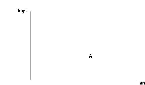
Assuming the person likes both logging and preservation of habitat, any combination (such as B) that gave more of both would be preferred; any combination (such as C) that gave less of both would be less preferred (the dotted vertical and horizontal lines through A mark the current amounts of logs and animals).

Preferences get complicated when we ask how a person would trade off one good for another. What increment more wildlife habitat (more animals) would balance slightly less logging? Call this point D. What increment more logging would balance slightly less habitat? Call this point E.

Connect together these points into a smooth curve, which we call an "indifference curve" because the person is indifferent between the various options.

One person's preferences might look like this:

which implies that this person likes both logs and animals. Indifference curves above are preferred; indifference curves below are less preferred.

Different people might have different preferences. This person likes animals and cares very little about logs:

While this person cares about logging jobs and not much at all for animals or habitat:

Horizontal or vertical curves would represent complete lack of caring for a particular outcome. This might accurately represent the views of some people on the extremes.

Why do we usually sketch the indifference curves as bowed? This is again an assumption about behavior on the margin. Return to an individual with preferences that are not too extreme,

From a point in the middle, such as point F, the person might make an almost equal tradeoff – a 1% diminution of habitat for a 1% increase in logging (for instance). However as the person moved upwards and leftwards (toward G), they might want a greater compensation of logging increase for equal diminutions of animal habitat. If there is a giant park then people might be willing to allow logging in a few areas but as the size of the wilderness shrinks, they become less willing to give up the remaining bits. Oppositely as the choices move from F toward H: more and more habitat is protected and so becomes less valued. This is the principle of diminishing marginal utility. (Diminishing marginal utility is the idea that, when I'm thirsty, that beer tastes great; when I've already had a few, I don't get quite as much enjoyment from one more beer.)

Note on Aggregating Preferences: although we derived a market demand curve from individual demand curves above, aggregating indifference curves is not so easy (in fact it's generally impossible!). Aggregating PPFs is simple, though.

Optimal Choice

Make the (not entirely serious) assumption that we have some units to measure "animals" and "logs". Starting from a value of zero logs and all animals, suppose we reduced the number of animal units by one? How many more logs could we get? This gives the opportunity cost of the last unit of animals.

But compare this high cost with the cost (in log units) of reducing the amount of animal, if the amount of animal is already small:

Somehow the society must figure a way to bring these two considerations of production possibilities and choice into equilibrium, to find the tangent of PPF and indifference curve:

A rational maximizing individual who does all of the production by him or herself, and knows his or her own indifference curves, would make this choice. In a world where production and consumption are separated, each side sees only the price,

So producers see only the relative price of a to l but choose optimally; consumers see the relative price and also consume optimally.

Consumer Choice and Fees/Taxes

There may be cases where policymakers are reluctant to impose fees for worry about the distributional impacts. For example, water pricing may lead to more efficient outcomes but this could lead to the poorest people suddenly facing a steep price hike for a necessary good. A gas tax, carbon emissions permits, and other programs all have this feature.

The simple way to fix this is to rebate the tax revenue to each person (but regardless of how much was purchased). It might seem that this would undo the effect entirely but with some basic micro we can show that although the increased income will stimulate spending on the good , nevertheless the price rise will diminish spending (this is the Slutsky decomposition of substitution and income effects).

Consider a typical consumer who chooses between good X and good Y (where Y is a composite of “all other goods”). Assume the price of Y is $1 and the price of X is P. The consumer has income of M. Then her budget constraint looks like this:

x

x*

And assume she chooses the point, (X*,Y*) as indicated.

Now a tax of T on good X would result in a rise in the price of X to (P + T) and shift her budget set inward, getting her to a lower utility level:

Now suppose that some of the revenue from this tax were rebated, to raise the person's income from M to M' to make the old X*,Y* just affordable.

Then the person is no worse off but still is using less of the good x – through only the substitution effect not the income effect.

Further refinements could adjust the marginal prices so that, for example, the first few units are available at a low cost while remaining units are more costly. This would provide people with a minimum level of the good without substantial deleterious effects on efficiency.

Appendix: A reminder about Percents and Growth Rates

A percent is just a convenient way of writing a decimal. So 15% is really the number 0.15, 99% is 0.99, and 150% is 1.50. When you remove the " % " sign you have to move the decimal point two digits to the left. This can be particularly confusing with single-digit numbers where the decimal point is at the end and therefore omitted: 5% represents the number 0.05 and 1% represents 0.01. If there is already a decimal point then it moves two places: 0.5% is therefore the number 0.005. In Macroeconomics this can get confusing since US inflation data is commonly reported as, for example, "0.2%" last month. This means that typical prices increased by 0.002.

If A is half the size of B then we can say that A is 50% of B. If it were a quarter of the size, it would be 25%. If a number is increasing then there are many ways of expressing this. Sometimes we say that Z is 125% as large as Y; this is the same as saying that Z is Y plus a 25% increase. You can see this from the decimals: 125% = 1.25 = 1 + 0.25, so it is equal to one plus 25%.

This can also get confusing when finding percentages of percentages. Many stores try to fool people with this: they offer "50% off and then take another 25% off additionally!" Does this mean that you get 75% off the regular price? No! Think for a minute: if they offered "50% off and then take another 50% off additionally," would that mean that they were giving it away for free? No, they're taking half off and then another half off – so you get it for a quarter of the original price (since ½ * ½ = ¼ or 0.5 * 0.5 = 0.25). So offering "50% off and then take another 25% off additionally!" means you get 0.50 off and then another 0.50 * 0.25 = 0.125 off, so the total is 0.50 - 0.125 = 0.375, which is 37.5% of the original price.

For instance, we might want to find 10% of 10%. We CANNOT just multiply 10*10, get 100, and leave that as the answer! Rather we first convert them to decimals and then multiply: so 0.10 * 0.10 = 0.01 = 1%.

So if I want to know, for instance:

· 4 is what percent of 25? I'd divide 4/25 = 0.16 so 16%.

· If some country has GDP of $125 bn and invests $33bn, what is its investment rate? 33/125 = .264 so 26.4%.

· A state had 47.3m jobs; employment grew at 2% so how many jobs does it have now? 47.3(1+.02) = 48.2 m jobs.

You can see from the examples that one of the other good things about percentages is that we don't have to worry about units. If the top and bottom are both expressed in the same units then the percentage is unit-less.

In economics the data are commonly used to try to persuade you to think one thing or another. Therefore, even if someone's not just outright lying, they're often telling you about the data in a way that persuades you one way or another. Whether it's stores and companies or politicians, they're trying to play with the data so you've got to be careful not to get played.

Here's another example. Would you rather invest your money in a bank account that paid 12% in interest each year; or one that paid 1% each month of the year? If you don't care about the difference then you're losing money. Take, for example, if you had $1000 to invest. If you invested it in the first account you'd end up with

1000(1 + 0.12) = $1120,

which is an increase of $120 in the year.

But if you got 1% each month, then after the first month you'd have

1000(1 + 0.01) = $1010.

This amount would be reinvested in the second month so you'd have

1010(1 + 0.01) = $1020.10.

Note that since 1010 = 1000(1 + 0.01), we could re-write 1020.10 = 1000(1 + 0.01)(1 + 0.01) = 1000(1 + 0.01)². So after three months you'd have 1000(1 + 0.01)³, after four months you'd have 1000(1 + 0.01)⁴, after five months you'd have 1000(1 + 0.01)⁵, and, well, I hope you can see a pattern. So after 12 months you'd have 1000(1 + 0.01)¹², which is equal to $1126.83. So you'd have $6.83 more after 12 months, if you invested $1000, which is 0.6% more. Sure, maybe $6 isn't a lot of money, but if you were working for a major financial institution with $10m, then that's $68,300 in a year. A person could live on that.

It should be clear that you've got to be clear about percentages and growth rates.

Generalizing to Formulas

Suppose you've got some amount of money, $Z, to invest. Suppose that the money grows at a rate of r per time period (usually a year). So if at first you've got $Z then after a year you'd have $Z and $Z*r, so in total you'd have $ Z + Zr = Z(1 + r). If you re-invested this money for an additional year (two years in total) then you'd have Z(1 + r)(1 + r) = Z(1 + r)². After three years, = Z(1 + r)³. If you put it in for T years and keep on re-investing then you'd end up with Z(1 + r)^T. This is compound interest.

Compound interest is often referred to as one of the most important fundamental concepts in business. This is because of the way that a small initial amount of money can grow and grow, if left to compound over a long time period. For example if you're planning to retire in 40 years you might want to start saving now. Why start now? Because, if you can save just $1000 this year, then after 40 years you'd have over $45,000 if it grew at 10%.

We often might want to solve backwards: if I end up with some amount of money after a given time period, and I know how much I started from, what was the rate of growth? For instance, if I end up with $45,000 after $1000 grows at compound interest for 40 years, what is the rate of growth? [Ten percent.]

To solve these sorts of financial problems, you want logarithms. (Trust me – I know, you're asking, why could anyone possibly want logarithms?! Keep reading.) It makes the math simpler. In fact business applications like these were the main reason why logarithms were developed. If you remember your algebra, you know that figuring just (1 + r)² is a bit complicated since you have to multiply it out to get 1² + 2r + r². Doing (1 + r)³ is longer and (1 + r)¹² is just masochism. But log(1 + r)¹² = 12*log(1 + r). So solving backwards is not too hard if you take logs of both sides [I'm talking about natural logs, ln( ), not base-10].

In many business and economic applications, the time period is something other than years. It could be months or quarters or days or just overnight. (Did you know that there's a huge market for lending money just overnight? Why? Because night here in NYC is day in Tokyo or other financial markets, so that money is valuable.)

Although we developed the formula for the growth in a bank account, it can be applied to any variable that is growing at some rate. That could be inflation or GDP or just about any other variable that changes over time.

Suppose I've got some time series of observations of a variable, X. So I label these as X_t, where the t tells me what time unit. It might be the year, in which case I might have X₂₀₀₂, X₂₀₀₃, X₂₀₀₄, ….

The absolute difference is VX, which is given by VX_t = X_t – X_t-1. The percent change is %VX = .

Suppose that we have information that a company's sales increased from $50m to $60m in a single year. What is the growth rate? The change in sales is $60m - $50m = $10m, while the initial level is $50m so the percent growth rate is ($10m/$50m) = 0.20, or a 20% growth rate. This rate has no units – sales happened to be given in units of millions of dollars, but the 20% growth rate would be unchanged if the sales had been in billions or thousands; dollars or pesos or euro; tons or hours or cubic yards.

If you know calculus then you can read on; if not then come back once you've been enlightened:

A final note, since I mentioned logarithms, I'll mention their relationship to calculus and to percent growth, since so many students miss it: the derivative of the log of x is the percent change in x. Or using the notation of %VX to represent the percentage change in X, then .

Important Conditions for Competition

Depend on Secure and Complete Property Rights

property rights are completely specified
all property rights are exclusive (no externalities)
property rights are transferable and enforceable

In considering these necessities, recall Arrow's Theorem of Second Best: a system of property rights that satisfies most (but not all) of the conditions is not necessarily better than a system satisfying fewer conditions – counting up the satisfied assumptions does not measure how near are the outcomes.

Markets

Microeconomic theory proves the First Welfare Theorem, which guarantees that a competitive market economy (with complete property rights and no transactions costs) is Pareto efficient – meaning that we can't make any person happier without impairing someone else. This is a big reason why economists believe that markets are generally the best way to distribute resources.

In a perfect economy people don't need to understand all the implications of their consumption on different resources; they only need to know the price. The price is the sole sufficient indicator of scarcity. So much energy is expended by modern consumers trying to balance off different criteria, even for simple choices like a lightbulb. An incandescent bulb uses 'too much' energy relative to a fluorescent, but fluorescent bulbs usually contain mercury (hazardous disposal), other types of bulb might consume particular resources (rare earth metals) in being made. How ought consumers to trade off greater electricity usage versus mercury contamination? A consumer can be left swamped with information! But in a perfect economy consumers only need to look at the price. Clearly we don't live in a perfect economy.

Recall supply and demand graph, plus PS, CS, DWL, so competition maximizes total surplus.

In production, supply prices in a perfectly competitive industry are determined from the minimum point of average total cost – this is the long-run industry supply curve. Firms compete to supply each commodity for the lowest price, meaning that they try to economize on inputs (use the fewest and cheapest possible).

Externalities

Externalities are cases of imperfect property rights. If my decision to consume some item has an impact on someone else, then who owns that spillover effect? This can be particularly acute in trying to resolve intertemporal or intergenerational allocations – what if my decisions affect people who will not even be born until the next century?

(Paul Krugman blogged about Pigou, the English economist who first theorized about externalities.)

Examples. Smoking carries an externality: my choice to inhale smoke means that people near me will also inhale smoke. That consumption choice imposes a negative externality. Other consumption choices might impose positive externalities: economists have found significant positive externalities from education, so your decision to get more education will tend to raise the wages that your family and people around you will get. Externalities can arise from production as well as consumption. A factory belching smoke imposes negative externalities on those down-wind. A flower farm might impose positive externalities (more commonly, a beehive kept by someone who wants honey will have positive externalities because the bees can pollinate other flowers of fruits or vegetables). There can be positive or negative externalities; these externalities can arise in production or consumption.

Hanley, Shogren, & White quote Ken Arrow, that an externality is

a situation in which a private economy lacks sufficient incentives to create a potential market in some good, and the nonexistence of this market results in a loss of efficiency.

Each word is essential: "lacks sufficient incentives" makes clear that it's not necessarily about technologies but organizations, "potential market" notes that even a possible market has effects (threat of entry or calls/puts), and the final phrase makes clear that not every market failure is insoluble and requires government action.

A a lack of a positive externality can be considered a negative and vice versa.

Negative externalities of production produce marginal external costs (MEC) above Marginal private costs (MC, the supply curve). Since these MEC are external to the firms they do not enter into a private firm's calculations of profit maximization so the private firm produces until P=MC. But this creates a deadweight loss since at this level the total social costs (MSC = MEC plus MC) are greater than the price, which measures the marginal benefits that people attach to this good. So it costs society more to produce than people value it, which is DWL. Graphically,

So in this case government intervention can reduce or eliminate DWL. A tax that is just equal to the MEC, or a regulation that limits industry output to Y*, would reduce the DWL to exactly zero. Consumers should pay more, P*, since that is the true cost. These taxes are called Pigou taxes after the economist who proposed them originally.

Examples of marginal social costs over and above the marginal private costs are pollution. Decades ago, a firm generating waste might simply dump it into the nearest river. This raised costs for other firms downstream if they needed clean water. (Where by 'firms' I'm including government operations for instance drinking-water treatment plants.)

Externalities loosen the case that individual maximization behavior will inevitably lead to social maximization. Consider the simple case of conversation at a party or bar: you want to talk with someone but there's so much noise that you have to speak loudly to be heard. As everyone in the bar makes this same choice, the general level of noise must rise and so everyone must, again, choose to speak even louder.

Generally externalities break down the argument that all government intervention must produce deadweight loss. Of course government actions are determined by politicians and so are often heavy-handed or even completely wrong, but this must be determined carefully and on the particular facts of each case. General statements, of the sort that politicians and newspaper editorials make, that all taxes are bad or all regulation is wrong – these statements are pure foolishness.

This is the basis for economists suggesting, for example, higher taxes on gasoline. Greg Mankiw, who advised President G W Bush, has a "Pigou Club" of economists lobbying for higher fuel taxes for just this reason (http://gregmankiw.blogspot.com/2006/10/pigou-club-manifesto.html). [Note: Mankiw is a clear communicator, which got him into trouble, since his views about the advisability of a gas tax, plus his views that 'outsourcing' is not really a problem, didn't mesh with that administration's overall message. I can disagree with him on many policy issues but still admire him for being intellectually honest in this case even when it was not in his best interest!]

A positive externality in production would shift marginal external costs to the right of marginal cost, creating a different DWL triangle because there would now be insufficient production.

Sometimes government intervention in "strategic industries" or to subsidize R&D is justified by this argument. Any single firm might have relatively high costs but the total social cost is lower, so government intervention (subsidizing production) might be justified.

Research into some area, say the basic biological science behind pharmaceuticals, is expensive. There are important knowledge spillovers so a breakthrough in a particular area is likely to lower costs for the whole industry. If you've had a class in Urban Economics you know that many firms choose their location based on these sorts of knowledge spillovers. Government-sponsored research in the San Francisco Bay area led to many hi-tech firms starting up there; now Silicon Valley is a highly productive location for a wide variety of tech firms. In New York, hip design firms choose to locate in areas where there is already a density of other hip design firms (Brooklyn or Tribeca or SoHo or wherever) – there are positive externalities to these locations that are not available in Flushing, or Newark.

Externalities in demand would shift the marginal social benefit curve to the left or to the right of the marginal private benefit (demand) curve. Positive externalities of demand are "bandwagon" effects or "network" effects – Facebook is popular because 'everybody' has a FB account so MySpace died (and Google + limps along). Negative externalities of demand are congestion effects – when the iPhone was introduced on AT&T's network, the huge demands for bandwidth slowed down everybody's phone. City traffic has this effect.

So in each case, a tax or price/quantity restriction can actually reduce the deadweight loss and make everybody better off.

Vertical Sum not Horizontal

Unlike the case of private demand where the market demand is the horizontal sum of the individual demands, the SMWP is the vertical sum of each individual's marginal willingness to pay (MWP). Because the nature of the externality means that the consumption is shared, we don't add up how many are demanded by each individual, at a given price. Rather we ask, if society were to consume one more unit (such consumption would be shared by many individuals), how much each individual would be willing to pay – and add up each individual's marginal willingness to pay.

These items can be positive or negative: I might be willing to pay something for public consumption of some good, or I might be willing to pay an amount to avoid the public consumption of that good.

Rival and/or Excludable Goods versus Pure Public Goods

A problem with providing public goods is that everybody tends to wait around for someone else to do the hard work. The idea is that, if the problem impacts somebody else, then that person might do the hard work and then I can just take the externalities – get the benefits without any of the costs. For example the global campaign to restrict carbon emissions suffers from this free rider problem: every country wants the other countries to take all the pain.

We can generally distinguish goods as either excludable or non-excludable and either rival or non-rival (in any combination).

Excludable goods mean that the technology exists to keep other people from using my stuff – kids fight in order to make their toys excludable, a mass of laws against theft and robbery help me keep my stuff excludable. Non-excludable is the opposite: I can't keep people from using it. Perhaps it's an architecturally lovely building that every passer-by can enjoy. Or the neighbor without curtains. Intellectual property law exists to try to make certain goods excludable.

Rival means that someone else's consumption of the good interferes with my own. If someone else eats my cookie then I can't eat it – cookies are rival. Non-rival is the opposite. Sometimes these distinctions are a bit arbitrary: parents don't understand why kids can't share toys, "If you're not playing with it now, why is it a problem if the other child plays with it now?" just like many people would consider their jewelry rival (even though the same argument could apply – but almost nobody, really, rents jewelry for a night out. The bling is only valuable if it's yours.).

Economists label goods that are non-rival and non-excludable "pure public goods." These are often goods that are provided by governments. Police and fire protection are difficult to exclude (both because of externalities) and, given the infrequency of occurrences, are basically non-rival. There are private security guards but these are not as common as police. National defense is non-excludable and non-rival.

But other goods, which the US government does not often produce, are also non-rival and non-excludable. Radio is – my listening to a particular station does not impact your listening (assuming the volume levels are low enough). (In other countries radio is produced by the government; in the US there is a modest subsidy to public radio.) Record companies and software companies are battling (mostly, failing) to make music and software excludable – even though any teen-ager with internet access can rip and burn music. Certainly it is non-rival, since I can copy a single mp3 file as many times as I like, without impairing my own enjoyment of it. The movie studios are terrified that their output will go the same way once users get enough bandwidth to easily swap movies peer-to-peer (since BitTorrent and similar apps haven't gone mainstream).

While these goods are not provided publicly, their peculiar character means that pricing must take different forms. Radio stations play advertisements if they broadcast for anyone; satellite radio makes their product excludable by encoding the broadcasts and selling the decoders. You can think of many more examples.

But in general, whereas we were able to prove the First and Second Welfare Theorems, in the case of no externalities and perfect property rights, to show that private markets produce Pareto-optimal outcomes, this is no longer the case when there are externalities or imperfect property rights. Markets are best wherever possible but they are not always possible.

This does not mean that every externality demands government intervention! Markets are dynamic and give participants incentives to figure out ways to exclude rivals, as the examples above clearly show. TV stations originally broadcast over the airwaves to everyone; now cable and satellite broadcasts require de-coders. Music companies are slowly trying to figure out how to exclude copying of their products (or figure out other ways of getting revenue – right now ringtones are supporting the labels!). Internet radio like Pandora or last.fm are complicating; Apple's iTunes store crunches the music companies' margins but offers greater security.

There are also cases where private citizens will join together and voluntarily restrict their own choices. Buying a coop or condo means that you agree to be bound by the decisions of a managing board, exactly in order to keep others from imposing externalities on you. If one person doesn't maintain his unit then the board has a legal basis to force the owner to make improvements. Business Improvement Districts (BIDs) have some of this character.

Free Rider Problem

People have an incentive to 'free ride' on other people's willingness to pay. Each would want the other consumer to pay more. I might claim that, actually, my preferences are not like my neighbor's; my neighbor cares greatly about the quality of the public good while I hardly care at all – so my neighbor should pay most of the cost. My neighbor, of course, will likely make the same claim.

Consider common debates about public taxation levels. Some people want the government to levy higher taxes and provide more services; others want lower taxes and fewer services. (In defiance of the facts, the former group would more commonly be associated with Democrats and the latter with Republicans.) Sometimes lower-tax supporters will assert, "Well, if you want higher taxes, why don't you start by volunteering to pay more tax yourself?" The public good argument and marginal-willingness-to-pay argument shows why that argument is fallacious.

This problem, of consumers having an incentive to "fake" their marginal willingness to pay for an item, does not occur in the case of private goods, because for ordinary goods, if I don't pay the price I don't get to consume the item. If I go to the coffee shop and offer just 20 cents for a cup of coffee, they won't give it to me. But with a public good, I have an incentive to try to get my neighbor to pay for the public good so that I can consume it for free.

Advanced: The Consumer's Problem for the case of Externalities

Economics investigates many cases of externalities; some of these relate directly to the environment. My decision to purchase organic food might help the people who live near the farmer's fields (which no longer are sprayed with dangerous chemicals). Or externalities could relate to networks or other non-environmental issues.

But for now consider two consumers choosing between two goods, x and y, where y is a pure public good (define) that would only be provided by some external organization (like a government). How much of the public good should be provided? Or, equivalently, how much would the two people be willing to spend?

This decision can be enormously complicated if we worry too much about income effects and complementarities among goods. If the free public goods are mp3 files of top music, provided by the internet, then my marginal utility for these goods might depend quite heavily on my possession of an iPod or computer. More seriously, there has been a lengthy debate on the degree to which people demand environmental services as they get wealthier.

But for now we start simply and work our way up. For any ordinary good we can graph a consumer's demand curve: the marginal benefit gained by consuming one more unit of the good. In general this demand curve will slope downward due to diminishing marginal utility.

For a public good we can ask the same question: what is the marginal willingness to pay by the consumer for a one more unit of this public good? Again, this will generally slope downward.

This can be again caricatured as the demand curve for the public good, although it has significant differences from a typical demand curve – crucially, that payment for public goods can be difficult to arrange.

One utility function, which is easy to work with, is the quasi-linear utility, where x is typically interpreted as a composite good (a basket of ordinary consumption items) with price normalized to one and y is the public good, so that and .

The marginal condition, that , gives once we substitute in for each term, where p is the price that people would be willing to pay for the public good (not necessarily the price that they actually pay). Take the marginal condition and simplify to get or ; the graph looks like the "Marginal Willingness to Pay" above [assuming the person has adequate budget to buy it]. There is an inverse relationship between the amount of the public good consumed and the marginal value attached to it.

Note that this is not the total value attached to the public good, just the willingness to pay for an additional unit more – that's why it's called Marginal. This is just the same as the case with ordinary private goods: the fact that I willingly pay $1 for another cup of coffee does NOT imply that I would give up all of my coffee intake for $1, only that my caffeine consumption is already high enough that I would only pay $1 for yet another cup.

Now suppose there were two people who could consume this public good. How much would these two people be willing to pay for this public good?

We figured out a relationship for the first person, , where p₁ denotes the marginal willingness to pay of the first person, and p₂ the marginal willingness to pay of the second person. So if the government provided a unit of y, which was nonrival and so could be used by both consumers, then society would be willing to pay up to p₁ + p₂ (as mentioned, this is the vertical sum). If the two people had identical preferences then . Graphically, this is a 'vertical' summation: add up the amounts that each person is willing to pay and that total price is the marginal amount that society would be willing to pay.

From micro theory, demand curves for private goods are the horizontal sum of individual demands, not the vertical sum.

So we can graph this to the right:

This basic principle applies whether the public goods have positive or negative externalities. Basically, the lack of a bad thing can be considered a good thing, for example if trash piling up is a bad then we can redefine and set trash collection as a good (last year this was a pressing concern in Naples).

Of course this assumes that there is some way to get people to reveal how much they'd be willing to pay for these public goods. This can be difficult…

Person 1 would willingly pay 0.5 in order to get 1 unit of the public good, y – which assumes that the other person is also paying 0.5. If there is not a full unit of the public good provided then Person 1 would not be optimizing. Person 2 will get utility from the public good provided by Person 1, even if Person 2 contributes nothing.

Consider now the case of two consumers with slightly different preferences: now person 2 has quasi-linear utility of the form so that . Now the marginal condition gives and so the Social Marginal Willingness to Pay is , so that, for example, if y=1 then person 1 is willing to pay 0.5 but person 2 would pay 1. So society overall would pay as much as 1.5.

How could these two people find this out? They have no incentive to tell the truth because they have no way of finding out the other person's true utility function.

What levels would be chosen, if the people were choosing individually? For simplicity we'll return to the case of two identical individuals with , and . But now we differentiate between how the individual could get this 'y' good, since it is non-rival. Either the consumer could buy her own or she could just use what others have bought.

Notate the amount of the public good bought by an individual y; the amount of the public good that others have already bought is Y (capital letter). Each unit purchased costs price p. So an individual consumes an amount (Y + y) of the public good and (x - py) of the private good (since after paying for y units of the public good she has only that much income left over for spending on x).

With the given utility function this is , where the person is choosing x and y, so we need marginal conditions for these two goods but not for Y since this is not chosen. So and (where the latter term, -p, comes from taking the derivative, with respect to y, of x-py) and we set the marginal conditions as (as usual we set the price of the private good equal to 1) and so we get , which we simplify to get or , which we invert to find the demand curve, . But how much of Y will be produced? If we assume that all of the consumers are identical and that there are of them, then the other (n-1) will do the same as the person under consideration, so . Substituting in to find , the amount chosen in private equilibrium, gets so , which means that the total amount chosen is . (Note to those who know micro theory: yes, this is the Nash game solution.) Most worryingly, the amount chosen by each individual falls when there are more other people around, who I believe will 'pick up the slack.'

But how much would be produced, if the people could get together and agree on an optimal social amount (somehow read each others' minds to find out how much they'd be willing to pay)? Now people would maximize their utility, , but the price of Y is since all of the population will pay for an equal part of the total amount that is consumed. So now the marginal condition sets = so, the optimal amount chosen by the optimal social welfare maximization, is .

Compare this amount with the private solution amount to see that , which will be positive whenever -- i.e. it will always be positive for public goods! The divergence will get bigger for larger populations, as well.

So while there will generally be some private provision of the social good, this will generally be much smaller than the amount that would be socially optimal. And the size of this divergence will grow bigger when there are more people sharing the externality.

You should be able to do this same analysis with a different utility function, such as Cobb Douglas. For this, and , . For the private-provisioning case, , , (this looks really ugly but many of the terms cancel so it's not quite as bad as it looks).

In our society probably the most common method of determining optimal social policies is voting, which will not in general produce optimal results but might be satisfactory. Recall the Arrow Impossibility Theorem which stated that democracy is not rational; also Churchill's "democracy is the worst form of Government except all those other forms that have been tried from time to time."

If people's preferences have some homogeneity (they're not too diverse) then voting can even be optimal.

Society has created a wide array of institutions that counteract the problems that arise from externalities. At one point these were largely based on sociological mores and traditions. Now many are contractual; in some cases governments have stepped in to formalize particular legal constructions – from the modern corporation to housing co0ps, condominium associations, business improvement districts, and so on.

The formal analysis mirrors the Nash game of oligopoly: although each participant would like to buy more Y (or charge a higher price), they do not do this because they assume that others would not be so 'public spirited' as to also buy more Y (or charge a high price) so they compete.

It is like a Prisoner's Dilemma. Return to the case of two identical individuals with , and . Their social optimum is to pay 1 and get 1 unit of public good (assuming p=1; this is ). But if they choose individually then they'd each choose so there would be just 1/16 of this public good in total.

We could simplify this as a Prisoner's Dilemma:

	Person 2 Cooperate	Person 2 Compete
Person 1 Cooperate
Person 1 Compete

But we need to fill in the Utility values in each bin. We assume that each person has a budget of 1; the amount of good x that is chosen is simply the remaining budget. Setting Y=1 implies that each chooses y=1/2 so x=1/2 and =1.5. Setting y=1/32 so Y=1/16 means instead =1.22. But if the other person buys 1/2 then I buy (where y' is the other person's choice of y). If the other person sets y'=1/2 then I would set my own y at zero (can't be negative) so my utility would be 1.71; the other person's would be 1.21.

So this gets us this Prisoner's Dilemma table:

	Person 2 Cooperate	Person 2 Compete
Person 1 Cooperate	1.5, 1.5	1.21, 1.71
Person 1 Compete	1.71, 1.21	1.22, 1.22

So "Compete" is a dominant strategy. As typical with this analysis, it could be extended to multiple interactions, complete with reputational games, random strategies, etc.

Coase Theorem

The Coase Theorem specifies why we link transactions costs with imperfect property rights: in the absence of transactions costs, many imperfections in property rights (many externalities) will be properly priced and so may be produced at Pareto optimal levels.

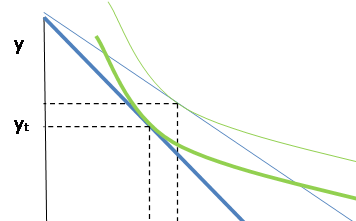
Consider the case of two neighbors sharing a building. One is a bar, which, in the course of ordinary business, produces loud music and loud people. The other is a laboratory which operates best without noise or vibrations; as these levels increase the lab must spend more money to shelter its experiments. Starting from zero noise, the bar gets a significant marginal benefit (MB) from the first few decibels of noise, however the marginal benefit falls as the level of noise rises. The lab can, with low cost, abate low levels of noise but its costs rise as it tries to abate more and more noise. Costs avoided are net benefits so we can consider this as a marginal benefit to the lack of noise: a small lack of noise has a small marginal benefit but as the noise rises the marginal benefit rises. So we can draw their respective marginal benefits (MB_L to the lab and MB_B to the bar) to different levels of noise (N):

Suppose that the level of noise were initially to be at some high level, N₁. Then the lab must be spending a large amount of money to abate the noise, MB_L(N₁), while the bar gets a much lower marginal benefit from the noise, MB_B(N₁).

If, instead, there were a low level of noise, N₂, then the lab could abate it at low cost, MB_L(N₂), while the bar would place a high marginal value (MB_B(N₂), a high marginal profit) for making more noise.

If there are clear property rights then the participants can trade. It may not matter if the law establishes that businesses have a right to silence or if the law establishes that businesses can make as much noise as they want – in either case the parties can then trade. If there is no clear law, either because there are no clear precedents or enforcement is capricious, then the two sides have an incentive to fight.

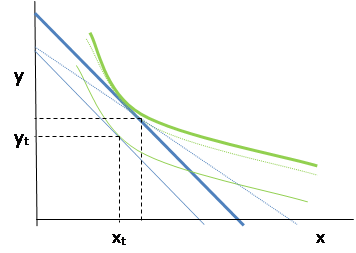
But suppose, for example, zoning laws mandate silence so that the lab has "ownership" of the lack of noise. In this case the lab can supply certain levels of noise by buying noise-reduction, so MB_L is a supply curve of noise. The bar would like to buy up the right to make a certain amount of noise, so MB_B is a demand curve. If we begin from cacophony, where the initial level of noise is at a high level such as N₁, then the lab would clearly want to lower the noise level: the last increment of noise could be sold at only a low price, MB_B(N₁), but it costs the lab much more, MB_L(N₁), to abate that noise. It will enforce a lower noise level. But not necessarily complete silence.

If, instead, the noise level were at a whisper, at an amount like N₂, then the bar would be willing to pay a large amount, MBB(N2), to be noisier, while the lab could abate that noise at a small cost, MBL(N2), so it would be profitable to sell the noise, buy the abatement technology, and make a profit from the difference. This will continue until the noise level reaches an equilibrium level, N*, where the marginal benefits to each side are balanced.

If, on the other hand, there were no restrictions on noise emissions, then the bar would have the right to emit as much noise as it chose. We can think of the bar as now supplying silence (the absence of noise, measured backwards on the horizontal axis) and the lab demanding silence. Since we're flipping the horizontal axis this gives a downward sloping demand (the MB_L) and upward sloping supply (MB_B).

If the amount of noise were at cacophony N₁, then there would again be an incentive for trading: the bar could make a profit since it could reduce noise at only a small cost while the lab would be willing to pay a large amount for that reduced noise. If the noise were at a whisper, N2, then the bar would find it profitable to emit more noise, and the lab could not "outbid" it since the bar would demand a high price of MB_B(N₂) while the lab would only be willing to pay MB_L(N₂).

The big insight is that no matter whether the lab has a right to silence or if the bar has a right to noise, the final amount of noise is unchanged at N*. The initial allocation of property does not change the outcome. All that changes is the direction of money payments: if the lab has a right to silence then the bar will pay it for the amount N*; if the bar has a right to make noise then the lab will pay it. The direction of the flow of money changes but not the amount of noise chosen. This was the insight of Coase. He did not believe that zero transactions costs were universal or even common, but his insight clarifies how the problems of externalities might be solved by private transactions.

Note that this result depends on the absence of "income effects" which, while reasonable in the case of firms (without financing constraints) might not be as reasonable for consumers. If poor people must buy a lack of pollution then they might not have enough income.

This also assumes that both sides to the transaction have continuous and monotonic marginal benefit schedules. If either MB curve were not continuous, i.e. with jumps, then the price might not be fully determined – but the two sides should be able to bargain. If either MB curve were not monotonic then there could be multiple equilibrium points, such as this:

So there can be many complications but the central insight is that we should concentrate on transactions costs.

From the Coase viewpoint, transactions costs are equivalent to unclear (or insecure) property rights. What would happen if, in the above example of the lab and the bar, the noise were made by cars going by (ones tricked out with the bass speakers thumping, or Harley motorcycles with their distinctive roar)? The lab would have a difficult time either enforcing silence (if it had that right) or paying the passing vehicles (if they had a right to make noise). Similarly if there is one noisy bar annoying large numbers of adjacent apartment-dwellers then it would again be difficult either for the neighbors to get together to pay the bar to lower the noise (if the bar had the right to make noise) or for the bar to compensate them each.

In air pollution discussions, this is the difference between "point sources" and "non-point sources" since point sources of pollution (like large power plants) are easily identified while non-point sources (like every car) are much more difficult to effectively regulate.

With unclear property rights, if the noise level just happened to be at N₁ but there could not be trading, then there would be deadweight losses equivalent to the shaded triangle DWL₁; if the noise just happened to be at N₂ then without trade the deadweight losses would be the other shaded triangle, DWL₂.

If the government can assign property rights to one party or the other then there will no longer be deadweight losses – i.e. there will be Pareto-improving trades. Alternately if the government knew the marginal benefit schedules of the lab and the bar, then it could regulate the noise level to be precisely N*. In the current case it would seem implausible that the government could really know all of that information, however in other cases the informational asymmetry might not be as large.

Steve Levitt (in his Freakonomics blog) gives the simple example of web addresses. For a simple example, consider the web domain name "kevinfoster.com". There are various people who might value this address (I checked – right now it's registered but just left blank).

Suppose I value the address at $100. Suppose that some business called "Kevin Foster" values the address at $120. If the property rule is "first come first served" and I was quick then I own that web site. So the business would offer me some price between $100 and $120, say $110, and we would both be better off – I would get $10 of surplus and the business would get $10 of surplus. Suppose instead that the property rule was "businesses get .com addresses" so that the business owns the web site. In that case they take it – I would not be willing to pay more than $100 for it; they would not sell for a price less than $120.

Suppose that, instead, I valued the address at $150. In that case, if I originally owned the name then I would keep it; if the business originally owned the name then I would buy it from them, for some price between $120 and $150.

In either case the entity that values the web address most highly will end up getting it – as long as they can make the transaction.

In the internet name case, the property rights were unclear initially: people named "McDonald" grabbed mcdonalds.com and demanded money. At first, the hippies who set up the internet tried to restrict sales, which just led to confusion. Businesses tried to use existing trademark protection law to grab domain names, so it took lengthy legal proceedings to figure out just who owned it in the first place. Once initial ownership was decided, trade could flourish.

Of course there are differences in the flow of money – if I already own the name then either I get paid (if the business values it more) or I don't have to pay (if I already own it). The participants in the transactions care greatly about the initial property rights allocation. But, as you recall from our discussion of Pareto improvements, from the point of view of maximizing surplus these transactions are immaterial. Neither is a Deadweight Loss – they're losses to one side that are gains to another.

Tragedy of the Commons

A particular case of an externality is called the Tragedy of Commons: when everyone can use a resource then they have incentive to over-use it. From the Coase perspective, the fact that "everyone" can use it creates substantial transaction costs.

Tim Harford, in his column The Undercover Economist, gives an example of popcorn during a movie. If a bunch of friends are all eating from the same bowl then the popcorn will disappear fast. If each person gets their own packet then they'll eat more slowly. I can save popcorn for the end of the movie if I have my own bowl/bag. But I can't save some if it's in the common bowl.

This was initially described as "Tragedy of the Commons" because in ancient times people grazed their animals on common land (a park in Boston is still called "Boston Common" from this). Since access was easy, the land was 0ver-grazed. It has other applications but particularly in things like access to common areas – fishing or hunting, for example. The ocean off the eastern coast of North America was once bountiful with fish; New York City's teeming immigrants were fed on Newfoundland cod. But those areas were overfished and the stock of fish crashed. Now tight restrictions are trying to allow those fish populations to recover.

Numerical Example: suppose a forest is used for hunting and the benefit that accrues to a hunter depends on the number of other competing hunters, so for example, with h being the number of hunters and B the benefit to any one, and the marginal benefit is . Graph is to the right.

If the marginal cost to each hunter is constant, say , then if the forest were managed by a single entity (person or corporation or government) then that person would allow hunting until , . However if there is no way of keeping hunters out then a hunter would enter as long as the average benefit (AB) per hunter, , is greater than the cost, so hunters would enter until . Comparing the two results we clearly see that in the first case, where the forest is managed by a single entity, , while in the second case -- four times the optimal amount!

h_tragedy

AB

c

h*

MB

h

From this it is straightforward to additionally note that, over time, the net increase or decrease in the available benefit is changed by different 'harvest' policies: over-hunting today (if h_tragedy is greater than the breeding rate) leads to lower hunting possibilities tomorrow, until the animals are killed off entirely.

Taking a larger look at the graph,

Clearly if MC is upward sloping then the difference between the "Tragedy" level and the optimal level would not be quite as large, but there would still be a gap.

The Tragedy of Commons explains traffic, too. Clear roads are over-grazed – too many people hunt down the quick routes.

The problem can be seen as unclear property rights: if I don't eat fast (or don't go hunting or don't go fishing or don't drive) then how do I keep a claim on the un-eaten popcorn (or un-killed game or un-caught fish or space on the road)? We will often return to the problem of unclear property rights (Coase transaction costs).

This simple analysis can be unduly pessimistic; in the analysis of Elinor Ostrom (who won the Nobel prize in economics in 2009) there is more optimism for the ability of communities to properly use common resources. Viewed by a political scientist there is more scope for the policies of a community to have an effect, compared with what simple game theory predicts.

In Ostrom's view (see her Nobel lecture for an overview), "humans have a more complex motivational structure and more capability to solve social dilemmas than posited in earlier rational-choice theory." Many public goods are provided by "polycentric" organizations (multiple government and non-government entities) that interact with other entities, individuals, and companies in complex and diverse settings, which end up often being more efficient than a single monopoly government. Her research focuses on "common pool resources" which are non-excludable but rival (although she does not like that terminology). She also distinguishes "toll goods" that are non-rival but excludable; these can be provided as for example toll roads or bridges or private clubs.

Ostrom rebukes economic theory for being myopic, "The classic models have been used to view those who are involved in a Prisoner’s Dilemma game or other social dilemmas as always trapped in the situation without capabilities to change the structure themselves. ... Public investigators purposely keep prisoners separated so they cannot communicate. The users of a common-pool resource are not so limited." Only in common pool resource "dilemmas where individuals do not know one another, cannot communicate effectively, and thus cannot develop agreements, norms, and sanctions, aggregate predictions derived from models of rational individuals in a noncooperative game receive substantial support." In more realistic and complex cases, property rights are not so clear-cut. Identifies at least 5 property rights to common-pool resources: access, withdrawal (harvest), management, exclusion, alienation (selling previous 4 rights to another).

In many respects the problem of Global Climate Change is a tragedy of commons: the atmospheric capacity to absorb CO₂ is a common resource available to every person on the earth. Can governments work together to " develop agreements, norms, and sanctions"?

Sustainability

It is difficult enough to figure out how some impartial policy analyst might measure social marginal cost or social marginal willingness to pay, when they differ from the private analogs, or what tax/subsidy would cure it. But that presumes that policymakers want to maximize social surplus. To what extent is that a good assumption? Is that sufficient?

First, how exactly do we (ought we) define Sustainability?

Sustainability and Sustainable Development

Principal definition from the 1987 Brundtland Commission, Sustainable Development is development that meets the needs of present generations without compromising the ability of future generations to meet their own needs.

At the American Museum of Natural History here in New York, the entrance rotunda has the following words carved into the wall:

Nature

There is a delight in the hardy life of the open.

There are no words that can tell the hidden spirit of the wilderness, that can reveal its mystery, its melancholy and its charm.

The nation behaves well if it treats the natural resources as assets which it must turn over to the next generation increased; and not impaired in value.

Conservation means development as much as it does protection.

Theodore Roosevelt, 26^th President of the United States (the youngest ever) and also a winner of Nobel Peace Prize, was a prominent advocate of conservation, wilderness, and the AMNH. The last two sentences on the wall can be seen as inconsistent or at least as implying different varieties of what we would now call "sustainability".

But Teddy Roosevelt's further quotes reveal more, "Conservation means development as much as it does protection. I recognize the right and duty of this generation to develop and use the natural resources of our land; but I do not recognize the right to waste them, or to rob, by wasteful use, the generations that come after us."

"Defenders of the short-sighted men who in their greed and selfishness will, if permitted, rob our country of half its charm by their reckless extermination of all useful and beautiful wild things sometimes seek to champion them by saying the 'the game belongs to the people.' So it does; and not merely to the people now alive, but to the unborn people. The 'greatest good for the greatest number' applies to the number within the womb of time, compared to which those now alive form but an insignificant fraction. Our duty to the whole, including the unborn generations, bids us restrain an unprincipled present-day minority from wasting the heritage of these unborn generations. The movement for the conservation of wild life and the larger movement for the conservation of all our natural resources are essentially democratic in spirit, purpose, and method." (Again, TR, A Book-Lover's Holidays in the Open, 1916.)

Sustainability, in whatever conception, is not straightforward to analyze within an economic framework. We need to work out the details of the definition farther.

Sustainability and Economic Growth

From J.C.V. Pezzey & M.A. Toman, (2008) "Sustainability and its Economic Interpretations," draft chapter in Scarcity & Growth in the New Millenium, ed R.U. Ayres, D. Simpson, & M.A. Toman.

Big question: can economy grow forever?

Sustainability in general is about equity between generations. Could either define it as equity of outcomes (utility) or equity of opportunities. If look at outcome, then ask: can future generations' utility continue without declining? If look at opportunity, then does wealth never decline?

Economic problem: in many analyses we assume that people discount the future – find the present discounted value of costs & benefits. We do this in analyzing investments by private companies as well as governments. But this discounting means that the welfare of future generations may not be highly valued.

Early papers on economic growth provide boundaries of the problem. If there is a depletable natural resource, then rational choice (discounting the future) by current generations implies declining consumption over time. (People do this just for themselves: many people don't save enough for their own retirement!)

If, on the other hand, technological growth is rapid enough, then the discounting dilemma is solved: consumption can grow over time. The discounting dilemma shows that, even if there are no externalities and every good is 'properly' priced, the economy might still be unsustainable.

First question: so what? If every current person likes the unsustainable path, then is there a moral basis to limit current choice? If so, who will limit current choices? Can we distinguish between people acting as 'homo economicus' in markets but as 'Good Citizen' in government? For a good review of how important is economic growth to basic human welfare watch Hans Rosling's TED talk.

Do people act rationally anyway? Do they discount in that way? How do we deal with the uncertainty inherent in some of these models? No easy answers.

Technology can allow growth but still there remains a fundamental question: if future generations will be much richer, then why must we now sacrifice for them? Why should the poor (us today) sacrifice for the rich (future generations)? (But note that ethical statement that rich should get less and poor should get more, is widely seen as having different answers whether the comparisons are intertemporal or at a single time.) Many countries and societies have developed by first exploiting natural resources to get rich, then only later remediating environmental harm (e.g. the USA).

The concern with subsequent generations is not new, of course. Read Edmund Burke, Reflections on the French Revolution, 1790, "Society is indeed a contract. ... it is not a partnership in things subservient only to the gross animal existence of a temporary and perishable nature. It is a partnership in all science; a partnership in all art; a partnership in every virtue, and in all perfection. As the ends of such a partnership cannot be obtained in many generations, it becomes a partnership not only between those who are living, but between those who are living, those who are dead, and those who are to be born." (Earlier in the same, he noted, "the age of chivalry is gone. That of sophisters, economists, and calculators, has succeeded; and the glory of Europe is extinguished for ever." http://www.bartleby.com/24/3/)

This question of discounting arises often in policy disputes. We will come back to it (esp. in climate change) but for now note that there is no simple answer.

Social Welfare

How can we, as economists, say much about which outcomes are better than others, with a minimum imposition of our own particular ethics and morals? Some outcomes might deliver high income inequality; some might constrain inequality but with a lower average level of consumption. How can we say which is better?

I'll use the general term "government" but this refers to any joint decision making body. People get together to form various organizations, which then promulgate rules that bind the members – any of these organizations can be considered a 'government' from the view of social welfare analysis. A building coop is a 'government' of a sort: it makes rules that (hopefully) help the people who live there. Business Improvement Districts join up local merchants. There are unions and farmer marketing boards. Then there are myriad levels of government in the conventional sense of the word.

So how can a government choose its goals? One of the very minimal items that we might propose, is that we ought not to omit any movements in allocations that are "Pareto improving." A Pareto improving trade gives something for nothing – someone gets more utility without anyone else getting less utility. Certainly these sorts of trades ought to be made, right? So a "Pareto optimal" economy has eliminated all of these possible trades and has no more possibility of getting something for nothing.

This is what kids do after getting Halloween candy: the one who likes chocolate best will trade away the Starbursts and gummi bears to friends who like those more than chocolate. Everyone wins.

The First Welfare Theorem of Economics tells that every (frictionless) market equilibrium is Pareto optimal. This tells us that, based on the rather meager definition of "optimal" that we just gave, that each market equilibrium meets this low criterion. This is nearly by definition: if there were some trade that would make both parties happier, then they would make it in a market economy (unless constrained by some friction; e.g. the whole Coase discussion).

The Second Welfare Theorem of Economics is more interesting. We just said that "Pareto optimal" is a weak condition – a dictatorship where one person has nearly all of the wealth, while the others toil in peonage, could be Pareto optimal. There are many possible Pareto optimal equilibria. Suppose society had some idea of which particular one it wanted – could a market economy get us there? The Second Welfare Theorem tells that every Pareto optimal allocation is a market equilibrium that started from some initial endowment. So this makes a lovely separation: if policymakers want to change which allocation they desire, then they ought to change the initial endowments. The market system is not the reason for inequalities or injustices – these mirror inequities in the original allocations.

But, as we said, there are many Pareto Optimal allocations – this is one consideration but not the sole consideration. How can society choose the "best" outcome? The Second Welfare Theorem said that, if we had something to aim for, we know how to hit it. But what do we aim for?

Not every Pareto Optimal allocation is very good: if we start from an aristocratic society with 1% of people getting nearly all of the wealth while the other 99% live at subsistence level, then there is no Pareto improvement that will help the 99% who are peasants without taking something away from the aristocrats.

We would like to have some sort of society utility function, analogous to an individual utility function, so that we could use the rational choice apparatus to look at social choices. Call this a "Social Welfare Function," denoted W( ).

One idea for a Social Welfare function is Utilitarianism, originally due to Jeremy Bentham, which holds that we should just add up the utilities of the people in the society, u₁, … u_N. This sets

, or, with slightly more generality,

where the a_i are weights. This has problems, chiefly being the impossibility of measurement, then the impositions upon human rights.

Remember from our definitions of utility functions that these are just arbitrary functions which represent preferences; any monotonically increasing function of a utility function is itself a utility function. One person's utility of chocolate could be 1,000,000,000; another's could be -1 but we CANNOT conclude that the first person likes chocolate better. How can we compare happiness levels?

Then there is the problem of human rights: if we believe that people have "certain inalienable rights" then the utilitarian framework could justify, say, selling one person into slavery if the money raised can make others happy enough.

The philosopher John Rawls proposed a minimax function,

He propelled this function by arguing that most people's definitions of a fair allocation depend upon their knowledge of their own situation: someone who is intelligent might happily agree to a society where smart people are well rewarded; someone else with different advantages would argue for a different allocation. He proposed a thought experiment: what allocation would be chosen, if the members of society could get together before they knew what their own situation would be – whether they would be fortunate or unlucky, healthy or sick, endowed with which talents? They would have to make a decision from behind a "veil of ignorance" over their future endowments. Rawls argued that, from this perspective, a person would give a great weight to the worst possibility – extreme risk aversion – that a society with substantial inequality would not be appealing because even a small chance of being utterly destitute would be too large. Therefore he proposed a minimax principle, that every change in allocation, away from perfect equality, must help the worst-off person. So he would allow greater rewards to, say, doctors, in order to give them incentive to help the sick and the most fragile members of society.

These social welfare functions so far allow people's utilities to depend on anything and everything. We might further restrict that people's utilities depend only on their own consumptions, in which case we would have a Bergson-Samuelson welfare function. But this is not generally realistic.

Rights-based social welfare functions run into difficulties since these generally do not allow tradeoffs – a slight diminution in some right might make everyone better off. But rights-based are generally "lexicographic" preferences where no positive benefit can possibly compensate ("lexicographic" since Azzz is alphabetized before Baaa). Yet different people have different ideas about which rights are most important (in the US, the Supreme Court must adjudicate when there are competing rights clashing). Many people voluntarily surrender certain rights in order to gain other benefits (e.g. a coop or condo association restricts property rights but is beneficial to property values); it is unclear why a social welfare function should not do so.

We might hope for an answer like "democracy". But Ken Arrow (CCNY alumnus and Nobel Prize winner) showed that a democracy does not guarantee rational orderings of choices.

Arrow's Theorem states that if we desire:

Completeness: The social welfare function, W( ), is defined for all allocations,
The social welfare function is responsive to individual preferences,
It is independent of irrelevant alternatives (so if W(X)>W(Y) then adding a choice Z, if W(X)>W(Z), does not change the original ordering) (like Transitivity)
It is not an imposed dictatorship.

Then, if there are more than 3 choices, there is NO POSSIBLE Social Welfare function can be guaranteed to satisfy all four conditions.

People care about justice and fairness and other considerations. Too many policy debates result from arguing about proposals, where each side uses radically different definitions of these terms – what do justice and fairness mean? Economists have proposed some definitions.

The Second Welfare Theorem got us focused upon initial allocations, so we might wonder if that will help. Is a symmetric distribution, where everyone gets exactly the same bundle of goods, fair? If people's utility functions are not perfectly uniform then people will voluntarily trade among themselves, and we will move away from perfect equality. Is this desirable? Would someone envy another person's allocation? Define envy that person i would prefer j's bundle rather than her own. An allocation is equitable if none of the bundles are envied. Define a fair allocation as one that is equitable and Pareto efficient (i.e. nothing is wasted). Now it can be proved that if society starts from a symmetric distribution then the outcome of market trading will be fair, under this definition. (But the symmetric outcome is not generally fair.)

From the definitions of Pareto optimality, economists have often backed off to the measure, "Possibly Pareto Improving" (or Potentially Pareto Improving), to indicate that some policy could generate enough surplus to compensate the losers and still leave the winners with something. For example, a policy that gave A $100 while costing B just $40 would be Possibly Pareto Improving since A could compensate B the $40 lost and A would still be $60 ahead. This is the theory behind the general introductory lesson on Deadweight Loss (DWL) – that social surplus could be increased by enough to compensate the losers and still leave the winners ahead.

This sneaks back a bit of Utilitarianism into the argument – now we're comparing utilities but using the measure of dollars (marginal willingness to pay).

The problem with "Possibly Pareto Improving" policies is obvious: the "Possible" does not mean that it actually does occur! A policy that made Bill Gates $100 wealthier while making the poorest person $90 poorer would likely be condemned by a variety of social welfare functions. But it is "Possibly Pareto Improving" (even if it is improbable that it actually will be). Policymakers could justify a progressive tax on the theory that it distributes some of these Possible Pareto gains from the winners to the losers, but the connection between this progressive tax and other policies is often lost.

The typical economist's tool of "Cost-Benefit Analysis" has this same shortcoming. This would add up the marginal costs of some policy, add up the marginal benefits, and then make the change if the benefits outweighed the costs. Again this avoids all questions of who gets the net (social) profit! Cost-Benefit Analysis is the same as Possible Pareto Improving.

It is not clear how a society would choose sustainability over other social desires. Nevertheless, suppose it were – could we measure how sustainable a society is, or is becoming?

Measuring Sustainability

Define "Total Capital" as man-made capital (machines) plus human capital (knowledge and expertise) plus natural capital (from the ecosystem). Write

Often distinguish between "strong" and "weak" sustainability

- weak sustainability implies that total capital does not decline – but this can include cases where natural capital is used to increase human or man-made capital. This assumes that each type of capital is a perfect substitute for the other. Also assumes that there is some metric to convert all of the types of capital into a single unit (usually present-value money) – otherwise how to add up machinery and university degrees with coal fields, biodiversity, and clean water?

- strong sustainability implies that at least some component of K_N cannot fall below some critical value – there are threshold effects. Precautionary Principle follows. The Stern Report on Climate Change ended up using this sort of argument to overcome the disagreements about measurement that are inherent in the previous definition.

- Green Net National Product (GNNP) proposed to supplement GNP to offset the depreciation of K_Natural. Augmented National Income takes Green but adds in technological progress. Related is Genuine Savings, which gives net investment after depreciation of all of the capital amounts. So if Augmented National Income is not rising then economy is unsustainable.

- if economy has endogenous growth then this might be fast enough to overcome environmental degradation

- Other measures include "carbon footprint" (or other footprints) but these lack clear justification

Short Review of Production

Firms Choosing How to Produce

Assume that firms want to maximize profit, p, which is Revenue minus Cost. This is far from a perfect description of the world of course but it's a start.

Split the production decision into two parts: first, if a firm wants to make a particular quantity of output, what is the cheapest way to make it; second, how much output will a firm choose to make. This division allows us to focus on particular pieces first.

The first question – to make a particular quantity of output, what is the cheapest way to make it? – gives us the single essential number: the cost of that amount of output. The cost of this output is the only important item that the firm, when choosing amount of output to produce, needs to know. It does not need to know the quantities of inputs or relative costs. This split can also be thought of as reflecting a firm's organization: there is the corporate level that makes the decisions about how much product to make, if those output levels have a particular cost. Then these decisions are communicated to the plants that make the output, where each plant manager is told to make a particular amount of output, using the cheapest input mix possible. The plant manager doesn't need to know how a particular quantity of output was chosen; the corporate level doesn't need to know details of how that output is made, just the cost.

At this level we are not paying attention to questions of corporate structure. Given the decision structure from above, we might think of the plant managers as being a separate firm, outsourcing production. (A brand-name computer maker buys chips from a separate company; it doesn't need to know details of how the chips are made, indeed that might be a close-held secret. All it needs to know is the cost.) Our modern economy has many such firms providing corporate services, from high-level research down to the company cafeteria. The informational savings are immense: a firm doesn't need to know the details of how each input is made, it just needs to know how much they cost. If they want paper, they don't need to ask about how many trees grew for how long, they just need the cost per ream. (This is why central planning fails, since there are no prices and so no informational savings.)

We begin our analysis at the base, at the level of the plant, which is given an order for a particular quantity of output and must choose how to most cheaply make it. Again we divide the decision into two parts: first asking what is physically possible (what inputs can make the output) and then asking which combination is cheapest.

One Input

The simplest case is where one input makes one output, so we simply have . The marginal product of the input is how much additional output is made by adding more input, or , which is the slope of the graph. Assume that it is increasing, continuous and convex.

The assumption of being an increasing function (i.e. that ) is anodyne. Just as with utility, if output actually falls when inputs rise then you don't need an advanced degree to figure out that you should cut back. The interesting problem occurs when output could still be increased and you want to figure out if it is profitable.

The assumptions of continuity and convexity don't seem as obvious. But they can be solved if we think of the firm's problem over a slightly longer period. Suppose that a firm's underlying physical process of production is discontinuous: it takes at least 100 units of input in a day to make 100 output units, but less than 100 of the input just won't even start up the machine. Is the firm's production function to be considered discontinuous? Well what if the firm got orders for 50 units of output per day – what would it do? Clearly it could just run the machine every other day, and average 50 units of output with 50 units of input per day. If orders run at 80 per day then the machine is run on 4 out of 5 days, and so forth. Of course this assumes that the output is storable and that the time over which we are speaking is relatively short (more on this later). But the assumption is not too bad.

The convexity assumption comes by the same assumption. If the firm can make 100 output with 100 input then it could make at least half as much output with half the input. (On the graph, any chord drawn between 2 points will lie on or beneath the production function.) If there were non-convexities in the underlying physical process then, again, production could be structured to avoid these.

The convexity assumption is also why we often talk about a "Law" of Diminishing Marginal Product. It is reasonable to assume that the Marginal Product, , is diminishing (or at least not increasing) because if it were increasing then, as in the graph above, the firm would want to figure out ways to exploit this.

Clearly, assuming just one input to the production function is restrictive. I can't think of too many things that are produced in that way (except for the world's oldest profession). We want to consider multiple inputs.

More than One Input

We commonly limit ourselves to two inputs because that allows easy graphing and still gets to most of the complexities. But you should be able to see how the number of inputs could be increased.

Now describe the production plant with a production function where inputs are transformed into outputs by way of a production function: . We could imagine a wide variety of production functions but we assume that it has some basic properties. Note that, whereas in the consumer problem, we were reluctant to make restrictions directly to the utility function and instead discussed assumptions about the underlying preferences, that was because utility was un-measurable and only a convenient descriptive device. Production is more easily measured as long as there is some physical output: tons of steel or pairs of sneakers or casks of beer. So we make assumptions directly about the production function.

We again assume that the production function is increasing (so more inputs lead to more output), continuous, and convex (or something like convex). Now define each input's Marginal Product: , where we use the function notation to remind ourselves that the MP for each input is likely to be different, for different levels of each input. This is important – there are likely to be complementarities in production. The Marginal Product of one input is likely to depend on the levels of other inputs as well. (For example we often hear statistics that workers in third-world countries are not as productive as US workers – this doesn't mean they're any worse, just that they have different levels of other inputs.)

Again we assume diminishing marginal products, that falls as input 1 rises (holding constant input 2) and vice versa. This "holding constant" part is particularly important since, while in the long run we might be able to increase output by increasing both inputs, in the short run one input or the other is usually less flexible. Consider the typical office worker nowadays, who usually gets one computer. If a company hires more people without buying more computers, then the productivity of the new people (whatever their talent!) will be limited as they have to jostle for computer time. Similarly if the company got new computers without hiring new people – a few people might get multiple computers on their desks, and some might be more productive with those new computers, but not very much.

This is distinct from returns to scale, which asks what happens to output if all of the inputs are increased. Hiring people without getting more computers might not raise output much; getting computers without hiring more people might not raise output much; but hiring more workers and giving each a computer might still raise output. Diminishing Marginal Products for each input alone does not imply diminishing returns to scale.

To more formally define returns to scale, suppose a firm doubled its inputs, and ask what would happen to outputs? If output doubled exactly then a firm would have constant returns to scale (CRS). If output increased by more than double then the firm has increasing returns to scale (IRS). If output increased by less than double then there are decreasing returns to scale (DRS). To put this a bit more abstractly, we compare the output from doubling the inputs, , with twice the original output, . If then production is CRS; if then IRS; if then DRS. Or, more generally, for any scale factor , if then production is CRS; if then IRS; if then DRS.

Short Run vs Long Run

Often one input is more flexible than the other. This means that our analysis should distinguish between the short run (when one input is fixed) and the long run (when both inputs are flexible). Often we assume that labor is flexible and capital (the machines) are fixed since building, say, a new assembly line takes time. But other firms might have different rankings – universities have tenured faculty, many of whom have been there longer than some of the buildings on campus!

Profit Maximization

A firm's profits are revenues minus costs, so a firm selling n different output goods, each for price p_i, and using m different inputs, each with cost w_j, would have profit .

First note that the costs must all be put into the same units – dollars per time unit. Which raises the question, if a firm buys, say, a truck that is expected to last for 5 years, how is this cost compared against the daily wage of the person driving it? To answer this we suppose that another company were set up that just rented out trucks: it goes to the bank, gets a loan to buy the truck, and then charges enough per day to pay off the loan per day. We consider that, even if a company doesn't actually rent the truck but actually buys it, that it could have rented the truck. So the rental rate is the correct cost of that capital good. In the real world more and more companies are separating their daily operations from their loan portfolio and renting equipment. If you work at an office, you know that most photocopiers are rented. Airlines rarely own their own jets, they rent them. Offices are usually rented space. (Employees are rented, too!)

The companies have figured out that correctly measuring costs allows them to make better decisions. Capital goods which are owned and given away internally as if they had zero cost are not efficiently used.

Economists also measure costs differently from the way that accountants do regarding payments to shareholders/owners. If a public company has an IPO and sells its shares for $100 each, then those shareholders expect something in return. They expect that the dividends (and/or capital gains) will return them as much or more money as if they had invested their $100 in some other venture. So the company had better return $8 per year if the investors could have gotten 8% returns. An accountant would count this $8 per share as a "profit" but economists see that as a cost to be paid to shareholders for the use of their money (their capital). If the firm were to return just $6 then the shareholders would be angry and the firm would be in trouble; if the firm returns $12 then the shareholders are delighted.

So economists often talk about "zero profits" being a general case, which makes people wonder how much economists know about the real world since any business newspaper daily reports companies making "profits". But we're just counting different things. If the regular return to capital is 8% then, if the firm makes $8 that the accountants call profit, we call it a cost and report that the firm made zero economic profit.

Profit Maximization with One Input

This means

subject to . Hiring one more unit of input will raise the firm’s cost by; this one additional unit of input will raise output by and so revenues will rise (assuming no market power) by , which is the value of the marginal product. If then the firm should hire more inputs; if then the firm should hire fewer inputs; so in equilibrium .

Note that, if one input is fixed, then even the two-input model becomes, in the short run, just this problem of profit maximization with one input.

Firms of course look at the price that they actually pay, not necessarily the price that someone else thinks they ought to pay. For instance, before laws against pollution, disposal of a firm's waste was free – it just dumped the waste into a river or something. (Disposal is, in a sense, an input into production since the firm can't make more stuff until it cleans up from the day before.) So of course a firm would have no incentive to reduce waste. But once there were laws about pollution (e.g. Clean Air Act, Clean Water Act, RCRA Resource Conservation & Recovery Act, CERCLA Comprehensive Environmental Response Compensation and Liability Act - Superfund), a firm might have to pay a specialist disposal firm to take it away. Now there is a price on this input so the firm has an incentive to limit the amount disposed.

Profit Maximization with Multiple Inputs

Consider a firm which has multiple inputs available for making the output, each of which is useful and productive. Each input has a cost (or wage, if we extrapolate from the case of hiring workers) denoted w_i.

As with the consumer's diminishing marginal utility, we agreed that the firm faces diminishing marginal productivity; the production function is and the marginal product of each input is the partial derivative, . The firm is to subject to .

Also as noted previously, the fact that each individual marginal product is diminishing does not mean that production overall has diminishing returns to scale – where 'scale' refers to a case where all of the relevant inputs are increased. As a simple example, most offices generally operate with each employee getting a computer. Buying more computers without hiring more people might increase output, but at a diminishing rate; the same would hold true for hiring more people without getting more computers. But getting more of both could allow the business to expand.

The firm will maximize profits by choosing inputs such that (in the long run), the ratios of , marginal productivity per cost of each input, is equal. The explanation should, by now, be typical: if spending $1 more on input i increased output by more than spending $1 more on input j, then the firm should decrease spending on input i while increasing spending on input j. This will not only allow the firm to make more output more cheaply but also tend to bring down the marginal productivity of input j while increasing the marginal productivity of input i, so that in equilibrium we have .

If one input has a price which is increased (say, by some environmental regulation) then this input will be used less. This is the substitution effect (see from marginal condition).

There is also a Scale Effect. As the cost of production rises, the quantity of output demanded will fall, so fewer of all types of input will be demanded.

Also, if that input is non-excludable like polluted air or water, then other industries could see their costs fall, so input used more – a different substitution effect. Also a different scale effect.

Cost Minimization/Profit Maximization

The firm’s problem to maximize profits generates a dual (sometimes easier) problem, which is how to minimize costs subject to a constraint of making a particular amount of output. (The constraint is important, though -- if the firm wanted to minimize costs without that constraint, clearly setting y=0 would be best!)

If the firm wanted only to maximize revenue (or if the input were costless) then the firm would subject to . A "costless" input sounds crazy but remember that Mankiw says, "rational people make decisions on the margin." Zero marginal cost is not that unusual: it's the usual condition for media companies – they pay a big fixed cost (to record a song or make a movie or TV show), but then their marginal costs are about zero: one more iTunes download does not cost them much!

Marginal Revenue

To figure out this problem of zero marginal cost but changing revenue, we just need another definition. Marginal Revenue, MR, is the change in revenue per change in output, . If price is a function of the level of output (e.g. the firm has monopoly power) then MR can be a complex function. If the firm operates in a competitive market then the price is outside its control, so the increase in revenue from selling one more unit of output is the price, p.

But many firms have monopoly power. Consider a fashion label selling handbags. They want to sell more because that means more revenue. But they also know that scarcity has value: some designers sell in only a few select boutiques and can charge very high prices; other designers sell bulk quantities in department stores and cannot charge high prices. This is a very general problem.

A firm that wanted just to maximize revenue would expand production as long as MR>0 and only stop when MR=0, when producing more output would no longer raise its Revenue.

Most firms, however, do not simply care about maximizing revenue; they want to maximize profits. (Particular parts of firms, however, might want to maximize revenue: for instance, most sales people are paid commissions on the sales they generate not necessarily the profits. Countrywide got paid per mortgage regardless of quality.)

A firm that wants to maximize profits will also have to take account of Marginal Cost. It is also convenient to figure other cost definitions.

In a perfectly competitive environment the firm's demand curve is a horizontal line – the market price for this homogenous commodity. The firm can sell as much quantity as it can produce at that price. Lowering the price will not increase the amount sold; raising the price will stop all sales. This is an extreme assumption but, as you think about it, not completely unrealistic. One of the important points of any business plan for a new company is 'the competition' – what other firms sell and at what price. If my firm offers the same product then I can't charge a higher price. Of course my firm might charge a higher price and offer a better product, but this means that I'm selling a different output.

The business press sometimes discusses the "commodification" of different markets: for example at one point, when computers were new, the chips were quite different and there were many different prices; now that chips are standardized there is much less variability in price. Financial markets are commodity markets: nobody offers a "20% sale" on stocks or bonds! Markets are organized in order to standardize and "commoditize" certain products: e.g. the CBOT offers corn futures to deliver "5000 bushels of No. 2 yellow corn"; or "100 troy ounces of refined gold not less than .995 fineness cast as one bar or 3 one-kilogram bars"; the NYMEX trades gasoline "reformulated gasoline blendstock for oxygen blending (RBOB) futures contract trade in units of 42,000 gallons (1,000 barrels)" for delivery in New York.

This is not to say that the market demand curve is flat, just that the curve for the particular firm is flat. Another way of thinking of it is that the firm is such a tiny player in the whole market that it sees just a tiny piece of it, which is essentially flat. But even if there are a limited number of companies then a firm might still face a flat demand curve for its product based on the other's price. A final example: whatever I sell nowadays, I have to know what Amazon or eBay charges for it – most all of my customers will!

Hotelling on Resource Extraction

Hotelling result on resource extraction: for an exhaustible resource, the price must grow

at a rate equivalent to the market rate of interest, so if p is the price of this resource

and r is the rate of interest then , the price will grow exponentially. Why?

Arbitrage between risk-free investment (getting r) and keeping resource in the ground. Keeping resource in the ground returns , the percent increase of its price. Note that if extraction becomes more difficult (diminishing returns) then more investment is required to get the same rate of return so this will eventually become unprofitable, even when there is still some resource available.

Sadly, while the theory is elegant it does not explain markets for things like oil. It might be a better guide for natural resource managers of forests, though.

Prisoner's Dilemma and Cartels

In the past there have been instances when OPEC was able to successfully (from its perspective) raise the price of oil and increase the revenues of its members. Why don't they still do that? To understand their problem, it is useful to consider the "Prisoner's Dilemma" – which seems like a completely different topic at first.

Consider two accused robbers. The police don't have enough evidence to get them on anything more than minor charges (each would get 1 year in jail) but they try to get each prisoner to confess and accuse the other. The police go to prisoner A and tell him that he can get a reduced sentence (just 6 months in minimum security) if he gives them evidence to convict prisoner B (who will get 20 years). They got to prisoner B and make him the same offer. If both confess, each will get 15 years.

What is the likely outcome? Both prisoners are likely to confess. Why? Draw a table of their choices and outcomes.

	A silent	A confess
B silent	A: 1, B: 1	A: ½, B: 20
B confess	A: 20, B: ½	A: 15, B: 15

The key insight is that, no matter what the other guy does, prisoner A is better off if he confesses. If B stays quiet then A reduces his prison time from 1 year to 6 months; if B confesses then A reduces his prison time from 20 years to 15 years. Same for prisoner B.

You might at first think this requires that the prisoners be in separate cells but this is not required – they can meet ahead of time and strategize, it won't change the outcome. Of course they would lie to each other but they should each realize that they are being lied to. The key is that, although they would like to both stay silent, they cannot trust the other player to achieve this result (even though it would be optimal for them).

How is this relevant to the behavior of cartels? A cartel has the same basic pattern of choices. If there are 2 players (companies or nations) then each has the choice: restrict production or produce a lot. Restricting production raises prices and profits. But restricting production means not selling and so not getting some revenue – better if the other player restricts production.

Production Externalities

In the simplest case, we can examine a firm making a single private (rival and excludable) output and incidentally a single public (nonrival and nonexcludable) output (for now, we assume that this public good is disliked). An easy example could be a power plant which makes electricity and pollution. (Actually a variety of sorts of pollution, which affect different groups of people: carbon, mercury, NOX, and sulphur dioxide are the main ones.)

In this case the production can be shown as being like a production possibility frontier but with the pollution increasing along with the output, something like:

The firm can choose any combination of electicity & pollution within the light blue area. Clearly, however, the firm would be foolish to choose a point inside the area; the points at the dark blue line are efficient. These are the production possibility frontier. They are efficient because there is no way to increase the output of electricity without also increasing the output of pollution (this would not be true for points in the interior).

At any point along the frontier of production possibilities, we can define the marginal rate of transformation as the change in output of pollution per change in output of electricity – the slope of the line. With the notation of e for pollution emissions and y for the output of the firm, the marginal rate of transformation, MRT, here is , where is the function linking the amount of emissions generated as determined by the amount of output produced. We can think of electricity generation as transforming some amount of a public good (in this case clean, unpolluted air) into a private good (electricity).

This interpretation of the choice along the production possibility frontier as representing a choice of marginal rate of transformation allows us to compare firms and make statements about the relative efficiency.

Suppose there are two firms which, for some reason or another, have different emissions per unit of output. Graphically this would be represented as:

If they each produced the same amount of emissions, they would of course be able to generate different output levels, but their marginal rates of transformation would also be different.

Clearly the marginal rate of transformation of firm 2 is lower than the marginal rate of transformation of firm 1. This means that when firm 2 generates one more unit of output, it creates fewer emissions than firm 1 does. This means that, if firm 2 were to make one more unit of output while firm 1 made one unit less – keeping the total output of the two firms at the same level, the increase in emissions from the second firm would be (in absolute value) less than the decrease in emissions from the first firm. So total emissions would be smaller even though the output was kept constant.

Consider a simple numerical example, where but . This is plotted as:

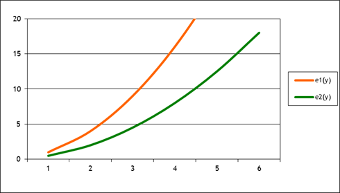
If emissions of each firm are 16, then firm 1 is producing 4 units of electricity while firm 2 is producing 5.66 units of electricity. If firm 2 produced one more unit of electricity its emissions would rise to 22.16, an increase of 6.16. If firm 1 produced one less unit of electricity its emissions would fall to 9, a decrease of 7. So if, instead of both firms producing 16 units of emissions, firm 1 produced less and firm 2 produced more, the overall production of electricity could remain constant while emissions fall.

We can continue this trade-off as long as the marginal rates of transformation are unequal. It is only when the marginal rates of transformation are equal that there will be a total efficient way of getting the most output with the least amount of harmful emissions. With a bit more math, we can find the point where the MRTs for each firm will be equal.

When we get to policy (next), we return to this idea: at the most efficient point, the marginal rates of transformation will be equal – which will not necessarily be the point where emissions are equal.

Hicks-Marshall rules of Derived Demand:

Demand for input is more elastic when

1. technical substitution is easy

2. input cost share is high

3. input substitutes are supplied elastically

4. demand for output is elastic

So putting the Scale effects and Derived Demand effects all together gets complicated. What is the impact of pollution restrictions on a firm, hindering its use of a particular dirty input? Clearly this adds to costs of the dirty input, but the impact of this cost change could be small or large depending on application of the Hicks-Marshall rules. Then what is the impact on other inputs (usually labor, i.e. jobs)? If the cleaned-up input is more labor intensive then this could mean a net rise in jobs; oppositely if the cleaned input is more capital intensive. If the cleaned input is more labor intensive, but the rise in cost greatly diminishes the demand for the product, then net jobs could fall if industry output falls. If the avoided pollution makes other factors more productive, then there could be further effects.

Might, for example, want to know the impact of a carbon tax on power plants. Here the share of inputs in total cost is clearly substantial; demand for output is inelastic – that's easy. Technical substitution is happening in the long term (few new coal plants, many more natural gas plants that are dramatically cleaner) but in the short term is limited. Input substitution is complicated in long/short run: natural gas production from domestic sites is increasing while facilities for imports are limited; oil is not much better; nuclear plants are tough to build; new hydro or geothermal is limited; other power sources are available but with limits (e.g. uranium production, solar panels now often imported, biomass facilities, etc.). Natural gas shows the inter-relationship of #1 and #3 in Hicks-Marshall rules: new gas turbines are relatively easy to install but if there is a rush of new construction then natural gas prices (which have recently moderated) will rise again and the cost advantage of natural gas over coal would erode.

Supplementary Material for Advanced students

Cobb Douglas Example

Consider a numerical example of a firm with a very simple Cobb-Douglas production function, so so the marginal products are (the last equation comes from a convenient simplification; it's a bit of a trick that's not obvious the first time you see it but you should be able to verify that it is, indeed, correct) and . The firm's cost is So put these expressions for the marginal products into the firm's marginal conditions that so so or . Put this into the production function to solve for so and -- these are the input demand functions, giving the firm's demand for each input as a function of both its output level and the relative price of the input. Put these into the cost function to find that the long-run cost is .

The long-run average cost is thus which sets the price in the market.

This allows us to easily see the scale and substitution effects. If the cost of an input, say w₁, rises, then this will mean that directly less of that input is used since ; this is the substitution effect. However it also raises the firm's average costs, in the long run so the amount sold must decrease. The size of this decrease in output depends on demand elasticity: if the output is elastically demanded then the price rise will produce a sizeable downward shift in quantity demanded.

Costs

The cost function is . It is determined, in the long run, by the wages of each input and by the level of output chosen. In the short run it is also determined by the amount of the fixed factor.

Marginal Cost is the change in cost per change in output, . Marginal cost is not generally constant but is commonly considered to vary with output.

We define several other costs:

Average cost, AC, is the cost per unit of output, . In the short run, some costs are fixed (F) and some are variable (.

Average variable cost, AVC, is the variable cost per unit of output, .

Average fixed cost, AFC, is , but since F does not change, this is just a rectangular hyperbola and doesn’t change much – so we rarely pay much attention to AFC. However we note that AC = AVC + AFC.

Also, from the definition of marginal cost and of fixed cost, we note that there is no need to define both marginal total cost and marginal variable cost – since fixed costs don’t change, marginal fixed costs are always zero so marginal total cost and marginal variable cost are always identical: .

These SR curves are typically graphed as:

Where we note that MC must intersect AC at the minimum point of AC; also MC must intersect AVC at the minimum point of AVC. To show this, note that by definition if MC>AC then AC must rise; if MC<AC then AC must fall. The minimum point of AC is where it turns from falling to rising, where it, for at least a short (infinitesimal) time it is neither rising nor falling so MC=AC. Same argument goes for AVC.

In the long run, there are no fixed costs, so long-run average costs (LRAC) are equal to long-run variable costs. LRMC are defined analogously to the short run.

LRAC can never be greater than the short-run AC curves – having more choices can never hurt profits!

In Long Run there are no fixed costs (can always choose zero output at zero cost). LR AC curve is envelope of SR AC curves – with a scalloped edge if there are discrete plant sizes but, as plant sizes become continuously variable, the LRAC becomes a smooth curve.

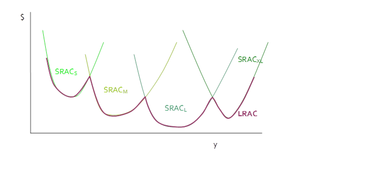
To maximize profit the firm will set . Consider this graph, where MR is allowed to vary as well as MC. To maximize profits, the firm wants to find where TR is farthest away from TC. The usual argument applies: making and selling one more unit of output raises revenue by MR; making one more unit of output raises costs by MC. If MR>MC then this was a good choice for the firm and it should raise output more. If MR<MC then this increased output was not a good choice and it should decrease output. It will stop this changing and reach equilibrium where MR=MC. In perfect competition where P=MR, this gives us the equilibrium condition P=MR=MC.

Profit Maximization in the Short Run

In the short run the firm must account separately for fixed costs. The profit maximization becomes: . Note that variable costs, , are a function of the level of output but "Fixed Costs are fixed." Fixed Costs don't change depending on the level of output, they're fixed. So the lowest level of profits that the firm could make are if output is set to zero (revenue and variable cost both become zero in that case). Beyond this, however, the usual rules apply. Recall that the marginal variable cost is exactly equal to marginal total cost. MC is how much cost increases when output increases. MR (which we assume to be in this case, for simplicity) is the amount by which revenue increases when output rises. Again, if MR>MC then the firm will produce more; if MR<MC then less.

So a firm with these cost curves (which we describe as canonical):

could face prices that lie in 3 separate regions: (A) either price intersects MC where MC is above AC; or (B) price intersects MC where MC is below AC but above AVC; or (C) price intersects MC where MC is below AVC.

Consider (A):

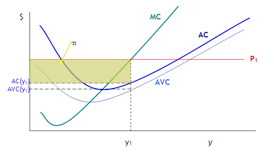
in this case, when price is at P₁, the firm will choose y₁ level of output to maximize profits. Profits are but can be more easily seen graphically as . So profits are drawn as the area of the rectangle with height and width , marked yellow in the graph. The decomposition of costs into Variable Costs and Fixed Costs can also be seen: VC are the area of the rectangle with height and width ; FC is the area of the rectangle with height and width .

With price at (B), where it intersects MC where MC is below AC but above AVC, we find:

Again the firm chooses the point where , which is . Profit here is actually negative, since , the firm's average costs are greater than average revenue. So the question arises, is the firm really maximizing profit? Well, what else could the firm do? It could shut down completely, but in this case it would lose , which, in the diagram, is again the area of the rectangle with height and width -- and this rectangle is clearly bigger than the actual profit lost. Basically, since operating costs (AVC) are below the price, it makes sense to operate even if the firm doesn't cover all of its fixed costs. It covers some amount of its fixed costs and so reduces its losses. This is just another manifestation of the old rule: sometimes the best that we can do still isn't very good. The firm is maximizing profits but still losing money.

Only in the case of (C) would the firm actually shut down. Consider:

Now with price at , the firm could choose to continue producing where , at the point labeled (from computer programming, the tilde means "Logical Not"). But at this point, the losses to operating, totaling would be larger than the losses to just closing down and losing fixed costs, the rectangle of area . So the firm chooses whenever the price is less even than average variable costs.

This tripartite division has many real-life ramifications. This is why hotels and airlines are willing to give last-minute deals: a butt in an airplane seat paying even $20 is more than the extra cost for the jet fuel to haul that little bit more weight. They try and try to charge more, to cover their fixed costs, but when it comes right down to the end they know that their variable costs are low.

Another ramification is seen in the housing bust. Driving through certain neighborhoods, there were still houses being constructed – why? Clearly the answer is that, since the builder has bought the land (usually the most expensive part), that FC is lost now. If a house sits half-built then the construction company loses all the costs put into it so far. But even if completing the building takes more expense, it might still be worthwhile – the builders will lose money, but not as much as if they walked away.

Firm Supply Curve

The firm's supply curve is then the locus of price and quantity choices, which is the firm's MC curve above AVC, then quantity jumps to zero if the price falls below this point. In the graph, this is:

Examples of tax affecting either FC or MC depending whether it is per production plant or per unit of output. If pollution is per output but tax/regulation is per plant, this could have mixed effects.

Choice of Dumping or Safe Disposal

( from Kolstad's Environmental Econ textbook)

Sometimes polluters face a choice of either cheaply dumping emissions (in a way that is socially harmful) or safely disposing of them. An example is garbage – it may be optimal to try to give households incentives to reduce their garbage by charging per pound or per bin, but this might also provide incentives for people to dump garbage in some deserted area. Consumers' batteries and electronic devices should be properly disposed of. This is especially relevant for producers who use various chemicals that need proper disposal.

One option is subsidizing the safe disposal, but this is costly and, of course, encourages more disposal. Suppose households were paid some amount of money per pound or per bin of garbage! That sounds crazy – but it might not be, if we can change other costs.

Assume a firm can dispose of waste, w, either, safely at cost or not safely at cost . Clearly there is only a problem if . So the government might introduce a subsidy per unit of waste, so changing the cost of proper disposal to (if the subsidy does not lower the cost enough then we're back to the original problem).

So how can we change other costs? Suppose the regulator observed the total volume of waste and taxed that, so now the costs for the firm are increased by but this is charged regardless of whether the firm dumps or disposes safely. The firm will not dispose safely if which clearly is no different. So the subsidy rate should be set to give an incentive to dispose safely while the net tax on waste, , should now equate to marginal damages.

A classic example of this is the deposit-refund system on bottles of soda, where consumers pay extra at purchase but then get a subsidy for proper disposal.

There are other examples of narrow-focused disposal charges, where buyers initially pay more and then can claim back some of this charge if the item is properly disposed (e.g. household electronics).

Regulation of Pollution

Command & Control

good because:

flexible in complex processes (law of unintended consequences)

more certainty for producers

bad because:

need so much information

low incentives for innovation

inefficient since generally violate equimarginal principle

Other refinements & policies:

subsidies might occasionally have some "bonus" or increasing returns provision, as with land use: a landowner who converts land to park gets more subsidy if it borders on an existing park; this is useful if the marginal benefits (to species habitat) are increasing in contiguous land area

from Law & Econ, we know that 100% monitoring is inefficient, better to catch some portion of offenders (e.g. 1 in 10) but fine them extra (e.g. 10 times as much) (see below)

could use "performance bonds" but these need careful monitoring (since generally forfeiture of bond involves lengthy legal proceedings); sometimes used on surface mining; also impose liquidity costs (extra financing needed) and open 'moral hazard' for regulators – 'pay-to -play'

Fees & Tradable Permits

A fee or tax per unit of emission is the Pigouvian solution – set the price and let firms decide. Tradable permits can give an equivalent outcome – permits are sold for a price; this price is essentially a tax.

Tradable Permits

Can easily show the financial burden on firms. Consider first the simple case: tradable permits sell for a price, P. At this price the firm chooses emissions of Ep.

Because, if the firm emitted more than E_p, it could cut emissions at low cost and sell permits at a higher cost; if the firm emitted less than E_p, it is cheaper to buy permits than cut emissions itself.

If the firm were given no permits at all, it would cost

Where the pink triangle is the cost of compliance: the emissions that the firm cuts back in response to the permit regime. The striped box shows the cost of buying Ep permits at price P. If the firm were given a few permits, E1, insufficient for its needs, then it would face the same cost of compliance but now:

Under this regime the firm gets E₁ permits and so only needs to buy the remaining permits, E_p – E₁. Or the firm might even get extra permits, which could reduce its costs below the cost of compliance:

Now the firm gets E2 permits, of which it sells off (E₂ – E_p) for a profit, which mitigates some of the cost of compliance.

If the permits are allocated only once (for example, when the policy is begun), then the dynamic effects of keeping unprofitable firms going (noted in the section on subsidizing firms not to pollute) will be small. If there are regular allocations of permits (yearly, for example) then these dynamic effects will be larger.

If the permits are given out in proportion to past emissions then firms will have an incentive to raise emissions just before the law goes into effect. Since many laws are debated for quite a while before taking effect, this is relevant. A law might have a multiyear lookback period.

Giving out permits in proportion to past emissions is also discriminatory to new entrants. If we consider policies like carbon permits to mitigate global climate change then this would mean that emerging economies would get fewer permits relative to richer countries.

Nonetheless giving out permits is common because it might make the program politically feasible: existing firms are given these valuable permits to get them to accept the new standards.

These worked really well, when US instituted tradable permits for sulfur dioxide (SO₂) in 1995 (see Schmalensee et al, Journal of Economic Perspectives 1998). They show this graphic, where the heavy line shows historical emissions per plant (sorted by level) while the light bars show actual emissions.

Clearly there was enormous variation: some plants drastically reduced emissions, far below what was required; others increased. The variation gives an idea of the scope of DWL from regulation.

Tradable Permits are usually allocated by either

- giving them away to current polluters (usually proportional to current pollution amounts, sometimes called 'grandfathering')

- auctioning them off to the highest bidder

A bit more Algebra

Suppose EPA issues L permits for pollution and each firm gets L_i

Firm emissions are and

Pollution, p, is , so

price of pollution is 

So firm's total cost is

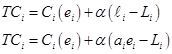
to minimize these costs set MTC=0 so

therefore

thus equimarginal principle is met

if there are multiple receptor standards, all of which must be met, then firms will choose e_i to meet the lowest limit

3 Results:

Equilibrium exists for any initial allocation of permits

Emissions from each source are efficient (no matter initial allocation)

If price equals marginal damage then equimarginal principle holds

Further details of cap-and-trade emission control systems:

- Only optimal for uniformly distributed pollutants – CO₂ leading to Global Climate Change is a perfect example

- For pollutants where the distribution is uneven, cap-and-trade could lead to more harm. If the plant with the highest cost to cleaning buys many permits, then its neighborhood will be highly polluted. However US experience with SO₂ has been reasonably successful.

- For non-uniform pollutants, the trading could be moderated by transfer coefficients (below)

- Depends on all actors being profit-maximizing – many polluters are government agencies, so this assumption might poorly fit particular cases

- If there are only a few firms, then the assumption of perfect competition becomes risible. One dominant firm could either get its permits cheaply or force competitors to pay extra.

- Transactions costs can also reduce the efficiency of the market

- So trading among zones or with complicated transfer coefficients has problems of both high transactions costs AND market power

When Costs & Benefits are Imperfectly Known (i.e. The Real World…)

Can think of regulation as either controlling quantity or price. Issuing a particular number of permits is setting the quantity and letting market determine the price of emission; a fee or tax sets the price of emission and lets the market determine quantity.

Need to consider:

§ whether there is relatively more uncertainty about marginal savings or marginal damages

§ whether marginal savings or marginal damages are relatively steep

Marginal Damages increase with the amount of pollutant, while Marginal Cost of emission reduction falls, since the first cleanup is easiest.

Extreme Case 1: Threshold effects of pollution

- virtually no damage below some level then damages jump to higher level once threshold boundary is crossed

Thought that MC was low at MC0 but actually is higher at MC1. A tax would have given P0; tradable permits would have set Q0.

So if costs of emission avoidance had originally been estimated to be MC₀ but were actually higher at MC₁, and if a tax had been set at level P₀, then firms, seeing this price, would choose Q₁ of emissions and we would have this case:

where there is now a HUGE deadweight loss: emissions are so high that marginal damages rocket upward – the yellow area shows the DWL of taxes set to the wrong level.

On the other hand, if marginal costs had been incorrectly estimated but policy had set a quantity target (number of tradable permits) at Q₀, then firms would pay a somewhat higher price and there would be a small DWL since the number of permits is slightly smaller than optimal:

Extreme Case 2: Constant Marginal Damages

- level of damage is nearly linear in amount emitted

probably reasonable in cases where, for example, damage is limited in geographical scope: ruining 200 acres of habitat is twice as bad as ruining 100 acres

So policymakers can regulate either the quantity (through issuing tradable permits) or price (with a tax on emissions). Again we ask, what if they are wrong in estimating MC? Suppose it's MC₁ not MC₀?

Then if regulators had set a level of tax at P0, then the quantity chosen would be Q1 with the new higher costs, so we'd get this situation:

Where there is a tiny bit of DWL (since MD might be slightly above the tax level, P₀) but this is quite small.

On the other hand, if the quantity had been regulated, then the prices of tradable permits would be bid up very high to P₁ since emissions abatement was much larger than anticipated, so we would have this case:

So here the DWL is much larger: firms ought to be allowed to emit more pollutant since their costs of abatement are so much higher than anticipated, but the stringent rule allows a sub-optimal level of pollution.

Neither of the extreme cases above might be likely in the world, but they're useful to pin down our thinking. When policymakers have a better idea of what is the optimal quantity (i.e. threshold), then they ought to regulate the quantity; if they have a better idea of the optimal price (linear damages) then they ought to regulate the price.

Case 3: MD steeper than MC

If the Marginal Damages curve is relatively steeper (less elastic) than the marginal costs of emission reduction, then we have a situation like this:

Again, if MC of emission reduction was incorrectly estimated and compliance is actually higher, then we have this case:

So if a tax had been set, the DWL would be the large pink area (from being too dirty); had tradable permits been set, then DWL would be the smaller orange area (being too clean).

Case 4: MD flatter than MC

If the marginal damage curve is less elastic than marginal costs, then we would have this case:

So if policymakers set quantity (Q₀) then they also get P_permits; if policy sets the price at P₀ then they get the quantity Q_tax.

So policy gets either of these two DWL areas:

So in this case, a tax would give a preferable result.

You might wonder what would happen in each case if the MD curve instead of MC were to shift, or if MC were to move down rather than up – I encourage you to sketch those out for yourself!

The general principle that we can deduce is that if policymakers are relatively surer about the optimal level of pollution, then tradable permits are good; if policymakers are relatively surer about the level of damage then a tax is good. Making good policy choices is tough!

Hybrid Price/Quantity controls might be better, to replicate the marginal net social damage, so for example a tax could be set but with an 'escape valve' that if the quantity of pollutants rose above some level then the tax would step up; or permits could be issued but again with an escape clause that if the price of permits rose above some level then more permits would be issued.

Details of Fees and Permits

Regulation of Quantity, in real world, must specify:

time of permit duration (daily, annually, etc)
information required
monitoring data to be provided
inspection schedule and costs of non-compliance (review Law & Econ result)
how often permit/fee will be updated

For dynamic efficiency, price regulation can be more effective than quantity regulation since there are better incentives for innovation – the price target is known so the marginal benefit to efficiency is known, which lowers the uncertainty of investment in efficiency.

basic model distinguishes sources and receptors, spread over space

emissions, e_i, from source any of I sources (plus background levels, B)

cause pollution, p_j, at any of J receptors

linearize for each j to get transfer coefficients, (valid in neighborhood if function is differentiable)

distinguish marginal damage of receiving p versus marginal savings of emitting e

Marginal Damage Cost, MDC, then is

Firms save money by emitting freely, so Marginal Control Cost

Social Optimum, (assume one pollutant) for each emission, i:

Pigouvian Optimal tax policy implies set therefore firms will choose emissions such that

What if different firms (firms with different transfer coefficients) pay same tax? Some inefficiency; size depends on elasticity of demand

If are the optimal amounts that emitters 1 and 2 ought to pay,

but instead the tax is set at , then the DWL is:

So efficiency depends on relative elasticities again.

Pollution Over Time

This analysis is for pollution that is transitory. However much pollution is cumulative: current emissions will pollute for a lengthy time period.

Model with stock of pollutants, St, the stock at time t, increased by current emissions, et, while some fraction () of previous pollutants decay.

S_t = S_t–1 + e_t

The Net Cost, NC is the present discounted value of all future costs of lowering emissions and all future damages from the stock of pollutants:

so the marginal net cost per level of emission is

where, from , we can re-write so that so .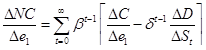

To minimize Net Cost, NC, set Marginal Net Cost equal to zero (the present discounted value of costs and damages equal to each other), which implies, notating and , means setting .

This can be interpreted as the marginal savings today should be equal to the sum of marginal damages in the future, where the future damages are discounted both by time preference and the persistence of the pollutant.

Of course for the case where the pollutant in completely transitory, so =0, this gives us the same formula as before.

Regulation through Liability

- more law & econ

Tort law (liability) involves the state setting rules to govern the behavior of 2 individuals, the injurer and the victim (technically, the potential injurer and potential victim, but for now we use the shorthand terms). Both may take a certain amount of care in their activities. For instance a manufacturer of a toy should take care that it not be dangerous; buyers should take care that it not be used in a dangerous way. Denote x as the care taken by the injurer, at a cost c(x). Often we might assume that the cost rises with x. Then denote L(x) as the loss to the victim; presumably it would be a decreasing function of x. The social objective function is to provide incentives for people to choose x to min c(x) + L(x). A typical analysis would show that the optimal level of care, x*, is where the marginal cost equals the marginal loss.

There are at least three possible sets of rules that would set incentives to each party:

No liability would give the injurer an incentive to minimize x, without regard to L.
Strict liability has the injurer paying all costs, so their costs are c(x) + L(x), so the injurer would take the optimal amount of care
Negligence, where the injurer is liable for all costs if he/she did not exercise “reasonable care”. If the level of reasonable care, x’, is set equal to the optimal level, x*, then this would provide the proper incentives again. If the injurer takes less care then they are back in the “strict liability” world where they pay the full costs; if they take more care then they have no gain; so they should set x = x*.

Up to now we have discussed care as taken only by the injurer. But now introduce care by the victim, y, so again there is c(y) the cost of the victim taking care and now L(x,y), where the loss to the victim depends on the care taken by each party. Now society wants to min c(x) + c(y) + L(x,y). Now there are two optimal levels, x* and y*, that set the marginal cost of care equal to the marginal diminution of loss.

Now the liability standards are:

No liability, so x=0 and y is too high.
Strict liability, where now the injured party has no costs so y=0 and x is too high.
Strict division of losses, where each side pays some fraction of the loss, f. In this case the injurer will min c(x) + fL(x,y) and so choose x to set MC(x) = f*ML, so x will be too low. Similarly for the victim, who will min c(y) + (1 – f)L(x,y) and will choose a y that is too low.
Negligence, where the injurer is liable if their care is below some x’ value. This must be analyzed as a game, since the outcome depends on the other actor’s behavior. We can see that the Nash equilibrium has each side choosing x* and y*. Suppose that the victim chose y* and the injurer is choosing. He/she knows that if care is too low then he/she will pay the full costs, so just as in the simpler case the injurer will choose x*. The victim will face the same choice: if the injurer chooses x* then the victim will be liable for the losses if y is too low; again the victim will choose y*.
Strict liability with defense of contributory negligence, where the injurer is fully liable unless the victim’s care was below some y’ level. Again, if y’ is set to y* then this gives an optimal outcome.
Double liability, where each side bears the full costs. The problem with strict division was that neither side took due account of the loss. If both sides pay the full cost, however, then both will take due care. This is useful in cases where the level of care is difficult to observe. It is the logic behind “no fault” car insurance where each party’s car insurance pays the bills and the traffic courts separately determine fault.

Regulation through Insurance

Insurance is intimately tangled with liability since often a firm, which is legally liable for some action, will buy insurance against that outcome (for instance, Director's & Officer's Insurance, which covers the company management from personal liability for their decisions at work). Workman's compensation is often used to cover liability to hazardous working conditions.

Insurance, to work well, needs six factors:

- risk pooling of

- clear losses

- over a well-defined time period

- that are frequent enough

- with a small moral hazard and

- small problems of adverse selection.

Note that "pooling" problems gave rise to reinsurance.

Valuation of Life

See Viscusi (1993) "The Value of Risks to Life and Health," Journal of Economic Literature.

Risk & Uncertainty

Risk is based on probabilities and can be treated mathematically

Uncertainty cannot be easily represented.

People are lousy even at evaluating risks, with little ability to differentiate between risks of different magnitude. That's why casinos can exist.

Behavioral economics has formalized some of these observations about how people are systematically irrational.

For a rational decision maker it is usually convenient to assume that an individual has von Neuman-Morgenstern utility. This means that a person's expected utility can be represented as:

. If a person's instantaneous utility function is concave then where we define the expectation operator as , X_i is the value that X takes in each case, and p_i is the probability in each case. The risk premium is the difference by which E(U) exceeds U(E).

This graph shows the case where there is either an accident (A) or not an accident (~A):

Often is convenient to suppose that an individual's instantaneous utility depends on two factors, income and some other event, some disaster. We assume that income is at level Y no matter which of the two outcomes occurs; then the other event is either A occurs or it does not (~A). Then utility is or . Evidently if the probability of A occurring is then the probability of A not occurring is .

Various measures of how valuable it is, to eliminate the uncertainty.

Expected Surplus

Define V as the amount of income which a person would sacrifice to be indifferent between having the full income and the disaster or having less income but no disaster. This is analogous to the Hicks measure of income effect that you learned back in baby Micro Theory. You might recall that this measure of income is not generally the same depending on where you start. In this case we must differentiate between utility starting from a disaster, , and utility starting from no disaster, . So define:

and

So the Expected Surplus, ES, is defined as the expected value of these valuations,

Option Price

Or the option price is the amount that a person would pay now to eliminate the uncertainty, so as to be indifferent between E(U(A)) and E(U(~A)). This option price, OP, is such that

Generally the option price will be larger than the Expected Surplus due to risk aversion.

Irreversibility and Precautionary Principle

Some decisions about the environment are irreversible, whether developing a wild "untouched" natural area or climate change that melts glaciers or loss of habitat that causes extinction of species. Additionally, there may be uncertainty about the valuation of these stocks: how much is a species worth, if we haven't even studied it yet?

This is called a "real option" in corporate finance (businesses confront these questions all of the time, investing in technologies with wildly uncertain outcomes). Waiting to make a decision becomes an investment in lowering the uncertainty of the outcome. A lower level of uncertainty has a value (from finance, people regularly trade off risk versus return, choosing for example between high-risk and high-return investment strategies or lower-risk and lower-return investments). So although making a development decision today increases the return (since the reward is closer to the present), delaying it brings a benefit of less uncertainty.

Actual Behavior of People making Choices under Uncertainty

People don't actually make choices in a way that adheres to these models; they're more complicated and irrational.

Kahneman and Tversky give these examples (from Kahneman's 2002 Nobel Lecture):

The Asian Disease

Imagine that the United States is preparing for the outbreak of an unusual Asian disease, which is expected to kill 600 people. Two alternative programs to combat the disease have been proposed. Assume that the exact scientific estimates of the consequences of the programs are as follows:

If Program A is adopted, 200 people will be saved
If Program B is adopted, there is a one-third probability that 600 people will be saved and a two-thirds probability that no people will be saved

Which of the two programs would you favor? Majority choose A.

Alternate Statement:

If Program A’ is adopted, 400 people will die
If Program B’ is adopted, there is a one-third probability that nobody will die and a two-thirds probability that 600 people will die

Which of the two programs would you favor? Majority choose B.

This is the "Framing Effect" and it has even been shown to affect the choices of experienced physician, depending whether treatments had a "90% survival rate" or "10% mortality rate".

Prospect Theory

Problem 1

Would you accept this gamble?

50% chance to win $150
50% chance to lose $100

Would your choice change if your overall wealth were lower by $100?

Problem 2

Which would you choose?

lose $100 with certainty

50% chance to win $50
50% chance to lose $200

Would your choice change if your overall wealth were higher by $100?

The choices are clearly identical but most people switch choices.

Can model people's utility as not from absolute level but from changes in wealth, and functional form is complicated:

"It is worth noting that an exclusive concern with the long term may be prescriptively sterile, because the long term is not where life is lived. Utility cannot be divorced from emotion, and emotion is triggered by changes. A theory of choice that completely ignores feelings such as the pain of losses and the regret of mistakes is not only descriptively unrealistic. It also leads to prescriptions that do not maximize the utility of outcomes as they are actually experienced – that is, utility as Bentham conceived it."

Most people make decisions based on simple heuristics, which are often approximately correct and are useful in minimizing the total mental effort of making a choice. Most people make choices about, say, what restaurant to choose for dinner tonight – not worth spending a great deal of time thinking about! They're not inclined to think much more deeply about bigger problems.

When college students are asked, on a survey, “How happy are you with your life in general?” and “How many dates did you have last month?” there is almost zero correlation; however if the survey asks them in the opposite order, the correlation jumps to 0.66!

The immediate corollary is that people can be cued to respond in a more statistically sound (rational or logical) manner, in ways as simple as just reminding them to "think like a statistician."

But it complicates the question of how we, as a society, ought to come to conclusions about complex issues involving a range of tradeoffs in the face of uncertain possible outcomes.

Basics of Oil

Many sustainability students would consider themselves opposed to fossil fuels. Nevertheless it is important to understand your opponent.

I can heartily recommend Jim Hamilton's papers as well as the book, Oil 101, by Morgan Downey, which is a great non-technical but highly informative read.

There is a myth that oil is made of dinosaurs – please discard this belief, if you want to be taken seriously! Oil is from fossilized creatures, but not the charismatic dinosaurs, rather tiny plankton and algae from ancient seabeds. Most oil is not from ancient fossils but relatively more recent (ie since the dinosaurs went extinct) less than 60m years. That organic material was buried under mud and sank downward, becoming kerogen (sometimes called source rock). As you know, the temperature of the earth gets hotter as you go deeper so the buried material, pushed downward, was cooked. There is a "window" in which oil can be formed – deeper forms natural gas. Much or most then evaporated up through the porous and permeable rock – oil and gas deposits are only found underneath cap rock, an impermeable shell that prevents these volatile gases and liquids from bubbling up to the surface, often shale or salt. Oil is often discussed as being in pools but it is actually in the pores of rock – which must be sufficiently porous (enough holes in it) and permeable (whether the holes are connected).

People noticed that there were springs with 'funny' smells or even tar pits, but this was a curiosity, not important to the economy, until Col. Edwin Drake struck oil in Pennsylvania in 1859. That began our modern era of petroleum fuels. While total US oil production increased steadily, this was a result of new exploration – existing fields were often quickly drained – many individual states hit "peak oil" and declined thereafter but total national production gained as new locations were found and new technologies allowed more effective drilling and extraction.

While oil drilling is sometimes celebrated as the free market in action, it was originally monopolized by Standard Oil (that built Rock Center), then much of the development of oil fields in Texas and Oklahoma was shepherded by strong government policy. Oil fields can be thought of as like a lake of water: a pipe in one place, pumping the liquid out, can drain away the liquid that other property-holders might believe is theirs. Property rights to the underlying oil were not clearly defined. Further, pumping too quickly (as from too many wells, all competing to suck up the oil first) could strand a large fraction of the oil. This is a tragedy of commons, of the type we discussed earlier. The Texas Railroad Commission (see Hamilton 2011 "Historical Oil Shocks") was formed to regulate and control the extraction, acting as a cartel with federal government support.

While the Suez Crisis of the 1950s left Europe without oil and encouraged more shipments from the Western hemisphere, there was not much of a world market for oil before the 1970s. A confluence of events in the early 1970s, including the ending of the Bretton Woods (gold-based) international payments systems, Nixon's wage and price controls, a peak in US oil production, and finally the OPEC embargo for the 1973 Yom Kippur War, led to the first modern oil crisis. Five years later the revolution in Iran led to another price spike. In the early 1990s there was another war in the Middle East that again spiked the oil price.

These are important for their relation to the US economy, "All but one of the 11 postwar recessions were associated with an increase in the price of oil, the single exception being the recession of 1960. Likewise, all but one of the 12 oil price episodes listed in Table 1 were accompanied by U.S. recessions, the single exception being the 2003 oil price increase associated with the Venezuelan unrest and second Persian Gulf War." (Hamilton 2011)

These graphs from Hamilton (2011) shows the historical oil price:

One common question is about "Peak Oil" – ever since M King Hubbert proposed an estimation in 1956 that production could be modeled as a logistic distribution curve; in 1956 he predicted the US peak of production. Estimates of the global peak are more difficult however, particularly in the face of expanding technology. One problem is that the data is so limited: although publicly traded oil firms such as ExxonMobil must publish their best estimates, most of the world's oil is controlled by national governments (NOCs are National Oil Companies) that treat even basic information as a state secret. Even statistics for the KSA's Ghawar field (the world's largest) produce more heat than light. All the oil majors distinguish between "proven reserves" that very likely could be extracted with current technologies at current prices, and "probable reserves" that are more uncertain. Although these estimates involve a degree of uncertainty, in the US the SEC has jurisdiction over publicly-traded companies. Nevertheless we can be certain that the world will eventually slow down the release of CO2 into the atmosphere, the question is whether this is done by deliberate policy in response to climate change or by a shortage of oil to burn. (See Hamilton 2012 "Oil Prices, Exhaustible Resources, and Economic Growth.")

While people work very hard to transform oil into a homogenous commodity, it does not start that way – every field is different, sometimes dramatically different. There are global standards such as WTI (West Texas Intermediate) or Brent Blend.

Crude oil is differentiated by a number of factors including density – how heavy the liquid is. The American Petroleum Institute created API density, ranging from zero to 100. Water is at 10°; lower numbers are heavier (the stuff used to pave the roads), up to 100° which is about 60% less dense than water (some could even be lighter than 100). Intermediate grades such as WTI, Brent, and even the so-called Arab Light are all intermediate density (in the thirties of API density). Venezuelan oil is heavy with API in the twenties (about 90% of the density of water). Oil sands produce oil about as dense as water. Of course much crude oil from the ground has large amounts of water – usually several times more water than oil is brought to the surface, so the oil must be de-watered.

Crudes also vary by sulfur content – "sweet" refers to oil with low sulfur, and "sour" has high levels. Sulfur is a pollutant and also corrodes equipment so it reduces the value of the oil. There are many other characteristics – oil is as varied as the life that produced it.

Refining is a very complicated process where plant operators look at the grades available (at various prices and delivery times) and figure out which outputs to make. Some refineries have a wide array of technologies to produce many different types. But the heart of refining is simply heating the crude in a tall tower and letting the vapors rise to different condensing trays – the lighter outputs go to the top and the heavier products barely rise. Light products are gases like methane and propane; then gasoline; then kerosene, diesel and heating oil, motor oil, down to grease/wax, bitumen (what roads are paved with), and coke (a solid burned like coal). Since gasoline is more valuable than many of the heavier products, those can be "cracked" into gasoline with heat and pressure. The "refinery gain" shows that they produce a greater volume of output than the heavy dense input going in.

These various types of products are then blended together to suit the market. You might be familiar with octane ratings for a car – higher octane fuels generally have less energy density but can be better compressed without igniting (knocking) so more can be injected, so the engine can be more powerful. Lead is a cheap way of boosting octane.

Oil exploration uses a variety of tools including "thumpers" where sound waves are bounced off deep rock formations.

As for getting the oil out of the ground, you can explore that in more detail by looking at BP's Deepwater Horizon disaster. The National Commission's Report to the President, "Deep Water: The Gulf Oil Disaster and the Future of Offshore Drilling," is here, http://docs.lib.noaa.gov/noaa_documents/NOAA_related_docs/oil_spills/DWH_report-to-president.pdf. Chapter 4 gives most of the detail of the drilling process and what went wrong; really though the entire report is worth a careful read.

Background on Global Climate Change

I expect most students know most of this but I give a quick review just to make sure.

The three most important aspects of global climate change are:

Human activity is changing the earth's climate.
The poorest people will bear much of the burden and the costs of this climate change.
As poor people become richer, this worsens the pace of climate change.

Note that #2 and #3 are contradictory – this is one of the reasons why there is no clear or easy solution. Part #3 also helps understand why predictions of the future are so difficult: different development paths can mean huge swings in carbon output.

For point #3, note that the easiest way to 'solve' GCC problems would be to reincarnate Mao and put him back in charge of China to impoverish a billion people; also reincarnate Nehru to put him back into India to impoverish another billion – poor people have a small carbon footprint! If you think that those seem like bad policies then we need to consider alternatives, of how people can become better off without polluting so much.

Part 1: Human activity is changing the earth's climate

Climate science gives insight about the role of carbon dioxide (CO2) in regulating our planet's temperature. In earth's lengthy history (over 4bn years) the planet's temperature has fluctuated; glaciers have advanced (covering even New York City's current location) or tropical conditions have spread outward from the equator. Life has continued but in different forms with varied species expanding, diminishing, or becoming extinct.

All of human history has occurred during a recent period of relative cooling – we humans are attached to the particular climate that we've gotten used to in our short time on this planet.

from climateprogress.org, "Must have PPT #1: The narrow temperature window that gave us modern human civilization," August 27, 2008

The earth's temperature has been influenced by the quantity of certain gases such as carbon dioxide, through the "greenhouse effect." The greenhouse effect traps some of the Sun's heat within the Earth's atmosphere. The atmosphere is transparent to incoming solar radiation (in certain wavelengths); much of this is absorbed by the planet and some is re-emitted, usually at lower wavelengths such as infrared. Greenhouse gases (GHG) absorb some of this infrared radiation so the greenhouse gases can trap heat within the planet. Therefore as the amount of greenhouse gases such as carbon dioxide rises, the amount of heat trapped within the planet rises.

There is a positive feedback loop (which is very complicated to model) where warmer temperatures can lead to more CO2 emissions. Recall from basic science that CO2 is helpful to plants: they take in CO2, use photosynthesis to release energy from it, take the carbon (the C) to make the plant itself, then emit the oxygen (the O2 part). Kids wonder how a tiny acorn becomes a giant tree – it's carbon. Trees are mostly made of carbon that has been taken out of the air. This is one reason why planting more trees can help global climate change, since they take carbon out of the air. But eventually when the tree dies, the carbon is usually released back into the atmosphere.

But not always; some of the carbon might sink into a swamp, for example. Oil deposits are the carbon residue of ancient life: carbon was taken out of the atmosphere millions of years ago and hidden away deep inside the earth. Hidden, until humans extracted it.

Where does the increase in CO2 come from? Much of it is "Anthropogenic," thus the term Anthropogenic Greenhouse Gases – gases which are created by humans (have genesis from us anthro's). There is debate over precisely how much of the increase in CO2 is due to humans. However there is no longer any debate over the basic fact of rising average temperatures and that anthropogenic greenhouse gases make the temperature rise worse.

Temperatures, showing what models show would have been natural versus what is due to humans:

From IPCC AR5 Summary for Policymakers, showing 90% confidence intervals.

Note, however, that although greenhouse gases tend to increase global average temperature, we have stayed away from using the term "Global Warming" since not all parts of the earth are getting warmer. The climate is changing, and on average there is more warming than cooling, but there are some places that are getting colder. These parts are not necessarily the parts that need it, though! It seems that much of Antarctica is getting colder. For this reason scientists prefer the more precise label of "Global Climate Change" (GCC) instead of global warming.

Just as an increase in global average temperature does not mean that every location gets warmer, an increase in local average temperature does not simply mean that every day will be a bit warmer. There is a greater likelihood of high-stress events such as heat waves and drought. There also seems to be a greater likelihood of harsher winters in some areas.

An example of the complicated effects caused by GCC is the pattern of rainfall. On average higher temperatures mean more evaporation and more capacity for the atmosphere to hold moisture. This chart shows the areas of the globe that are predicted to get more rain (in blue) or less rain (in red).

From IPCC AR5 Working Group I Report

Looking closely shows that many of the areas that will get less rain are the areas that are already dry: the Mediterranean and northern Sahara, southern Africa, the US Southwest, and southern Australia. The human effects are disparate: in the US Southwest, people in LA and Las Vegas might have to conserve water better; in Africa many people who are already in poverty might face starvation as crops fail. There is some evidence that the conflict in Darfur was worsened by drought and competition for scarce water.

Part 2: The poorest people will bear much of the burden and the costs of climate change

As with just about everything else in the world, poor people will get the worst of it. This is true both across countries and within countries.

An example of the human impact of weather events was provided by Hurricane Katrina in New Orleans (although it was not directly caused by GCC). The victims were overwhelmingly those with the least income, the least political influence, and the lowest social standing. The hurricane caused significant economic losses but the wealthier people usually had insurance (which diffuses the costs). The worst effects and most deaths were among the poorest.

There are a host of other effects. The chart below shows the impacts on water availability, on ecosystems, food availability, coasts, and human health. Below the chart is a second graphic which shows the range of outcomes predicted by different models, with most showing a 2º-4º C rise in global average temperature (for Americans, this is about a 4º-7º F rise).

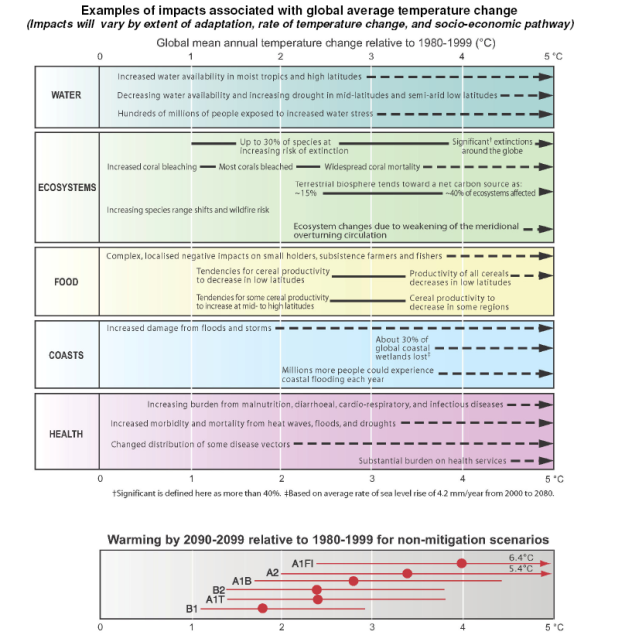
Figure SPM.7 from IPCC AR4 SYR SPM.

Water stress and the risk of drought is predicted to increase. The rise in average temperature not only changes patterns of rainfall and snowfall but also reduces the size of mountain glaciers. These glaciers act as reservoirs that release water into rivers slowly throughout an entire season rather than triggering flooding at spring thaw. Among the catastrophic outcomes would be if the Himalayan glaciers decreased significantly, since these feed rivers stretching through Pakistan, India, Bangladesh, Myanmar, and China. (Andean glaciers face similar threats.)

Ecosystems will begin to see a rising number of extinctions. Since the ocean absorbs some of the increased carbon dioxide, this change in its chemistry will have negative impacts particularly on coral reefs.

For food the picture is more complicated: colder regions at higher altitudes are likely to see increases in production for modest temperature rises – farmers in Canada and Russia win. However food production in countries nearer the equator will fall – African and India will lose. Again, this means that some of the poorest people on the globe will face threats to their basic ability to scrape a bare living.

Coastlines will see significant problems from the rising sea level combined with more rain and possibly more frequent or stronger hurricanes. The rise in sea level hits coastal wetlands which have an important role in water quality as well. Many of the world's cities (therefore a high fraction of population) are on low-lying areas susceptible to floods. Richer cities will build levees and dykes; poorer cities have fewer resources available. Within cities the richer people can move to higher land or commute, leaving the poor behind.

Finally there is the direct effect of disease changes from climate change. Again colder areas will see a modest improvement from fewer wintertime deaths but this is likely to be more than offset by more deaths from tropical diseases like malaria as well as heat waves.

The IPCC report notes that human societies have two main strategies against climate change: Adaptation & Mitigation.

Adaptation is taking steps to survive and prosper under new climactic conditions: society's stocks of capital were designed for particular conditions and rebuilding these is expensive. If roads near the coast need to be redirected, if subways and tunnels need new pumping systems, if water systems need more pipes, if flood protection needs higher walls – all of these substantial public infrastructure projects are expensive. While these projects are counted as adding to future GDP, they come at the cost of investing in other areas or direct consumption.

Humans have been successful in adapting to many different climates. But again the important note is that the rich and powerful will likely adapt easily; the poor and powerless will face huge problems. Poverty reduction goals set by the UN and other development agencies will be much more difficult to meet.

Mitigation is taking steps to reduce carbon emissions so that the Global Climate Change is smaller. Climate change has already begun; even if humans stopped emitting carbon now there is enough inertia that the average temperature would still climb more before stabilizing. The choice is not between Climate Change or no; the choice is how much Climate Change we are willing to accept.

Mitigation strategies must identify which industries and human activities emit the most greenhouse gases and then figure out which of these emissions can be reduced most easily.

One of the most important mitigation strategies is for governments to create the proper incentives, often to stop subsidizing harmful activities and to begin discouraging them (for example, coal mining is often subsidized by government policies).

The Stern Report clearly summarizes the common position of many economists that a carbon tax or a cap-and-trade policy, which can have identical effects, would be the most effective way to reach a targeted level of emission reduction.

These policies to reduce climate change will reduce GDP now and in the future. Larger reductions mean larger costs. Given the complexities of estimation of climate and economy, a cost-benefit analysis seems implausible. How complex? Consider the records of economic forecasters and weather forecasters; combine them. Seriously, it is very complicated because any scenario of future carbon emissions has to take account of how much carbon is emitted by the economy, which is going to be chosen by the society over the next century, as well as the future path of poverty reduction. (Poor people have few resources and so don't pollute much but a reasonable policymaker would want more richer less-polluting people.)

The particularities and the complications are innumerable; the field of climate science is still developing rapidly. Nevertheless the uncertainties in the science are relatively small compared with the uncertainties about human behavior in the future – the global climate a century from now will be most affected by policy choices.

The paper, " The Economics of Global Climate Change: A Historical Literature Review," by Stern, Jotzo, and Dobes, is a useful overview. Also the Stern Report and Nordhaus' replies.

Social Cost of Carbon

The Obama White House proposed a Social Cost of Carbon to be used in cost-benefit analyses.

Financial Markets

Financial markets for commodities such as oil can reveal important information about expected future prices.

These notes are based on John C Hull, Options, Futures, and Other Derivatives and Frederic S. Mishkin, The Economics of Money, Banking, and Financial Markets.

To understand the place and function of commodity markets, we need to start with a bit of perspective on financial markets overall.

Financial Markets and Securities

Financial markets are intentionally creating commodities, where these commodities are little pieces of paper representing legal claims to a particular commodity or cash flow (securities such as stocks and bonds). But then there are other derivative securities, with a value that depends on (is derived from) the value of another security. These securities can be for current transactions (spot markets) or transactions happening in the future (forward contracts).

Financial Markets trade money. If you only think of money as currency then trading money seems odd. But money is much broader. Financial markets allow me to trade money through time – if I have money now, I can turn it into money later; six months from now or 30 years from now. Depositors have too much money now; those who take loans don't have enough money now but will have money later. Financial markets trade money from different countries; euro to dollars to renminbi or many other transactions. Financial markets also trade money in different states of the world, depending if different events occur – contingent claims. Insurance pays only if some event occurs (if a person dies, the life insurance company pays money). Stocks pay only if the company makes a profit. Options pay only if a stock or other security has a value in some range.

Financial markets promote the efficient use of scarce capital by ensuring that firms with the most productive possibilities get investments. The broader the scope of individuals and firms that can get loans, the more likely it is that loans will be based on the merit of the project to be funded. Of course stupid ideas can still get funding, nobody is perfect! But this is the ideal. The problem is avoiding "dead capital" – saving hidden away, in case I need it in the future, but where nobody else can access it to invest.

Before there were organized markets, loans were made in individual transactions. But markets bring several advantages: standardized structures bring lower transactions costs (much of this through the legal accretion of case law) and a sharing of risks over more participants. The standardization brings enormous savings in solving some of the essential problems of giving money to someone else, whose incentives and information are quite different from my own.

Consider the problems that rich people would have without capital markets (in history, this is what was done). They want to make interest on their savings by loaning it out. But they would have to evaluate each borrower on their own and then monitor each borrower. Each lender would have to pay a lawyer to write up their loan contracts. In a large market there are economies of scale as well as liquidity services – if lenders get together then if one needs liquidity then she can get it.

This also makes possible risk sharing: if there are many lenders then losses can be spread over more of them. Eg: if there are 100 people each making a loan of $1000 then if 3% of loans are bad (no repayment) then any single lender has the possibility of a large loss. But if these 100 people get together and form a bank that makes 100 loans of $1000 each, then if 3% are bad then the bank loses $3000, so each person loses just $30 out of their $1000. Assuming they are risk averse, this outcome is much better! This may also give diversification, since an investor can avoid putting all of her wealth into one large project but instead put a little bit into many projects in different industries, to get a diversified portfolio.

Financial intermediaries also have a wider selection of tools to deal with information asymmetries (where one side of a deal knows more than the other), adverse selection (asymmetric information before the transactions), and moral hazard (asymmetric information after the transaction). Large financial institutions can screen out bad credit risks more effectively and monitor better.

Commodity Markets

People have been trading commodities for centuries; there were complex contracts involving future transactions in rice in Japan in the 1600s. Agricultural commodities are most common but there are contacts for many raw materials such as metals and energy, then weather, real estate, and financial commodities such as foreign exchange, interest rates, credit ratings/defaults, and stock indexes, even volatility on these.

Both producers and consumers want the widest possible markets: buyers want to find the lowest possible price and sellers want to find the highest possible price. A central commodity market makes it easy to shop around. In NYC there are many markets where both buyers and sellers cluster such as the diamond district or fashion district. Commodity exchanges provide buyers and sellers access to a large number of counterparties. They also have lots of people working in the middle.

The ability to buy and sell in the future helps firms on both sides. A mine can sell its output in advance, so that it will not be exposed to risks of its output falling in price. A manufacturer, that uses some input, can buy this input in advance and lock in the price, so that it will not be exposed to the risk of that input rising in price. For example, an airline might buy its fuel in advance so that it knows, when selling tickets to customers, that it will make a particular profit that is not put at risk by fluctuations in the price of jet fuel.

Most financial markets have hedgers (participants using the markets to reduce risk), speculators (participants looking to make bets) and arbitrageurs (market makers). (Details below.)

Commodities are traded in carefully defined and structured contracts. Crude oil contracts can be traded on CME (Chicago Mercantile Exchange) for delivery in any month from February 2013 to December 2018, and every six months until 2021. Each contract is for 1000 barrels (a "mini" is 500 barrels), with minimum movements of 1 cent per barrel (so the contract can move up or down by $10). That's a lot of oil! More than most backyard swimming pools. Average price in 2011 was $94.88 per barrel so a single contract would be worth $94,880.

Useful webinar from the CME on the Fundamentals of Energy Trading, http://www.cmegroup.com/education/interactive/webinars-archived/fundamentals-of-energy-trading.html

Futures and Options

Many commodities and financial instruments can be either exchanged now or a contract can be arranged for a future transaction.

Definitions:

Derivative: value depends on another variable; examples options (calls, puts, swaps, etc)

Forward contract: agree to buy/sell a particular asset at given price and date/time.

Spot contract: agree to buy/sell a particular asset at given price NOW.

Forward vs Future contracts: futures are traded on an exchange in regulated sizes

Valuation:

S_t is the value of some asset at time t (so S₀ is value at time zero, the beginning; S_T is time at time T, often expiration date)

F_t is the value of some forward price at time t (the price at time t, of some asset to be delivered at date T>t; sometimes for clarity denoted F(t,T) the value at date t, of an asset to be delivered at T.

For now we just take these prices as given: some trader or exchange tells us what the price is. (This is equivalent to saying that the financial markets are perfectly competitive so that our position will not affect the market price – we don't have market power.) Later we will ask what the prices, theoretically, ought to be. But first we have to understand the details of how portfolios can be constructed when the prices are just taken as given.

Long on forward: agree to buy at future date

Short on forward: agree to sell at future date

Exchanges vs Over-the-Counter (OTC): BIS reports that OTC derivatives have notional value of about $640 trillion while exchange-traded contracts were about $25 trillion. Commodities are smaller, just under $3 trillion, with gold about $0.5 trillion and metals $0.1 trillion. (http://www.bis.org/statistics/derstats.htm)

The particular price at which the option or forward trade will take place is Exercise Price or Strike Price (K).

The particular date by which the option or forward must be exercised is Expiration Date or Expiry or Maturity.

Payoff to Long position on a forward = S_T – K

Payoff to short position on a forward = - payoff to long position = K – S_T

Spot and Forward Prices

How can we develop a relationship between the current price of an asset (spot) and its future value? First we have to think about how these two prices are set. Clearly there is a relationship between them, but what?

Consider if the spot price were 100 and the forward price, for delivery in a year, were 110. Would you rather buy it now for 100 or spend a little more to lock in the price?

There are a couple things that we immediately notice we're missing. First, since we're comparing money in two different times, we need to worry about the relative values of these dollars – i.e. the interest rate, which gives the price of next year's dollars. We also need to know something about how/if the value of the underlying asset changes – if we're buying ripe tomatoes then they'll go bad long before a year is up; if we're buying oil then we have to store it somewhere; if we're buying stock shares they pay dividends.

Interest rate: assume the rate is given as "r" and that we're working in continuous time so the present value of each dollar, paid in a year's time, is e^-rT, where T=1 so it is e^-r.

In the example above, where spot is 100 and forward is 110, if the interest rate is low then we could borrow money today to buy at spot, sell it at the forward price, make $10 per transaction and if the $100 borrowed costs, say, $3 or $4, then that's a nice profit from the arbitrage. On the other hand, if the interest rate were very high then the opposite transaction would be more worthwhile. If I have $100 I could put it in the bank and get more than $110 after a year. Sell short at the spot rate (100) and buy forward at 110 to lock in the price at which I return the underlying asset. (Like Hotelling result for resources.) The difference (how much more I earn from interest over the 110 forward price) is arbitrage profit. In either case, the arbitrage trades work to change demand and supply to bring the prices back into line.

We might be confused because we might think that the forward price is a predictor of the price that will be set at that future date. But it's not – the spot price is a predictor. Why? Again, we consider what actions might be taken by a smart financial trader. Suppose that it is known that, on Friday, the price of some asset will jump from 50 to 75. Clearly, someone who holds the asset on Friday will get a huge return on their money. So what is likely to be the demand for that asset on Thursday? Wednesday? Tuesday? Today? The argument gets more complicated if the asset is difficult to store or if it changes value when held. (Under some circumstances, the futures price can be an unbiased estimate of the expected future spot price, but we still worry about the interest rate.) But the core arbitrage argument is clear.

These examples assume that the value of the asset does not change much over the time period. So we differentiate between an investment asset and a consumption asset. This tells if large numbers of market participants will be able to arbitrage (as outlined above) or whether large numbers will be eating what they buy. (I wouldn't sell short a forward for a pint of Ben & Jerry's because I'd eat it and wouldn't have anything to deliver at the end of the contract!)

In some way we can think of putting money in the bank as buying money forward: if I put $100 in the bank and get (without risk) some return, r, so that after a time of T, I get 100e^rT. This is like buying forward 100e^rT at a price of $100. Any other forward contract can be thought of as delivering in some different units of measure – but still, in the end, I should get the same rate of return. Whether I buy forward 1 gallon of crude oil, or some equivalent number of liters, doesn't matter. Similarly it doesn't matter whether I buy forward dollars or yen or euro or hog bellies or gasoline or S&P index contracts….

All of these arbitrage arguments get us to our first equation: F₀ = S₀e^rT, today's forward price is the future value of today's spot price. This is strictly true for investment assets in markets where arbitrageurs can borrow and lend at the same riskless rate, there are no transactions costs or other taxes, and there are enough (potential) arbitrageurs. You can think of it as just offering one more way to invest – you could get the riskless rate on the money or buy an asset that would (again, risklessly) provide some payment in a year.

Of course some stocks have a known income or known dividend yield, so we can modify the equation to take account of these complications. Other assets have storage costs (negative known income) or convenience yields. The convenience yield is defined as the amount that we observe that market participants are willing to forfeit in order to have the actual physical asset rather than a futures contract.

If we generalize about the "cost of carrying" some asset forward, whether that is the interest rate to finance it, or the interest rate less the income actually earned, or the interest rate less the foreign interest rate, or interest rate plus storage cost, denote the "cost of carry" as c so that for investment assets,

while for consumption assets, where y is the convenience yield,

Also there are many contracts that offer interest held in different currencies – again the same arbitrage arguments should hold. If I can risklessly get some r interest rate in US dollars then I should be able to lock in an equivalent rate in euro or yen or any other major currency. If I have a unit of foreign currency (FX) then I can either buy dollars at S₀ and invest in the US to get S₀e^rT at the end of T time, or I could invest the FX at the foreign rate to get and buy forward at F₀ to end up with F₀. Set these two end possibilities equal, S₀e^rT =F₀ or .

Next we move to valuing these forward contracts. The forward price is F₀ but the value of the futures contract (agreeing to buy at that forward price) is f. This sounds confusing but it is the simple result of the distinction between the value of a contract and its notional price – for example you could buy insurance that will pay $25,000 if you die – but you don't pay $25,000 for it! Of course a forward contract is not probabilistic – the whole point is that there is an ironclad agreement to trade at F₀.

Suppose for some asset the spot price is 100 and forward price is 110. If I enter into a forward contract that sets a strike price (denote it as K) of 110 then the value of this contract, f, is exactly zero. Tomorrow is a new day so the prices will change (but not K – that's written into the contract) and f = (F₀ – K)e^-rT.

You might be asking why anyone would enter into a contract where the value of it is zero. This is what arbitrage means – that although everyone is trying to make money, on net the prices must give no arbitrage profit. A significant fraction of the parties buying and selling are hedging: they're not looking for arbitrage profit but rather to lock in some price. (Also, leverage.) Later on, as the forward price changes away from the strike price, the value of the forward contract will change – that's the point.

Finally we discuss the relation between the current futures price (F₀) and the expected future spot price (E(S_T)). An investor might have some expected future spot price that is different from the market, so she could put the necessary cash in the bank today (cost F₀e^-rT) and expect to get S_T. However this expected rate in the future should be discounted by the investor's required rate of return given the risk (systematic or non-systematic) that she is taking on. But speculators would enter the market until F₀ = E(S_T)e^(r-k)T. If the asset risk is uncorrelated with the stock market, then r=k and F₀ = E(S_T). When the futures price is below the expected future spot price (so k>r) this is called "normal backwardation"; when the futures price is above the expected future spot price (so k<r) then it is "contango". (There are a number of linguistic theories about where that word comes from.)

Options

Call Option: the right (but not the obligation) to BUY a particular asset on or by a particular date at a particular price

Put Option: the right (but not the obligation) to SELL a particular asset on or by a particular date at a particular price

The asset, from which the option value is derived, is the underlying asset or underlier.

American vs European vs Asian options: American options can be exercised at any date up to the expiry; European options can only be exercised on the date; Asian options are exercised on the date but payoff depends on average price.

Puts and calls can be bought when they are "in-the-money," "out-of-the-money," or "at-the-money" (ATM). In the money means that the option would have value today given the current trading price; out of the money means it would have zero value if the expiration date were to be right now; at the money means that the strike price is just equal to the current price of the underlying asset. (so, for a call, S_T>K is in the money, S_T=K is at the money, S_T<K is out of the money; for a put S_T<K is in the money, S_T>K is out of the money, S_T=K is at the money).

If you think of these as being like insurance, then buying insurance against a flood, when the sun is shining, is buying out of the money. If you wait until the storm is washing up to your home, then you're buying in the money.

payoff to European call = max{0, S_T- K}

payoff to European put = max{0, K - S_T }

Positions Closed Out not usually delivered

As delivery date nears, futures price should converge to spot price

Futures contracts have daily settlement (so cash flows)

factors affecting option prices: strike, time, volatility, interest rate
swaps are based on interest rates, where parties swap rates, usually fixed for floating (often pegged to LIBOR, which had recent scandals that you might have read about)

Types of Trading

Traders are generally classified as:

hedgers – reduce risk of other positions
speculators – bet on market movements
arbitrageurs – make multiple positions and profit from the gaps

Hedge

A hedge is basically locking in cash flows at an early date before the asset changes hands. Consider a position, S_t, that will have value S_T at some future date, T. If that asset is hedged then a forward is sold at time T and bought at time t, so that the net asset position is S_T – F_T + F_t. We expect that, by the time of expiration, the spot and futures price will be equal (or else there would be arbitrage opportunities) so we expect that, by date T, S_T – F_T = 0. So the hedge is exchanging a volatile price (S_t becoming S_T) for a known price, F_t.

Short Hedge: own an asset and short a forward to sell at a pre-specified price.

examples: gold mines might sell the gold, that's still in the ground, at pre-determined prices at some date in the future to "lock in" a profit; farmer can sell the crop forward; exporter with short-term receivables might pre-sell (sell forward) to lock in a profit rate. Consider an insurer selling annuities in Japan that doesn't want the business affected by FX fluctuations so it could sell forward contracts for 3, 6, 9, 12 months (based on expected sales over the year). If these revenues are to be invested in, say, US Treasury securities, then these securities can be bought forward as well.

Hedge can be considered by comparing the money lost on the asset position with the money gained from the offsetting hedge. For instance, if the insurer above is getting ¥100,000,000 in 3 months. If the spot rate is 112¥/$ then this is worth $892,857.14. If the rate increases to 122¥/$ then this is worth only $819,672.13. The movement of ¥10 in the FX rate meant a loss of $73,185.01 on the asset position. If the forward price is also 112¥/$ then selling ¥112 forward (getting one dollar delivered in 3 months) would mean that, if the yen increased to 122 per dollar then the short forward position would mean that the company could sell ¥112 for $1 and still have ¥10 left over to buy dollars (0.0819 worth). This 8-penny gain is small compared to the $73,185.01 loss – but the company could sell more than ¥112. How many 112¥/$ contracts? 73,185.01/0.0819 = 892,857.14 worth (which is exactly the number we discovered earlier). This might seem like the long way to go about it but it is worth showing the basic method: one position loses a certain amount; it can be hedged if I can find some other position that would gain that same amount. Most companies use hedges with much more complicated structures, but the basic idea remains: construct two offsetting positions so that, as one loses the other gains (and vice versa).

Long Hedge: will buy an asset in the future and buy a forward to but at a pre-specified price.

examples: manufacturers that use mining products (gold, copper, etc) or plastics can buy in advance and lock-in their costs. Southwest Airlines made huge profits, compared with some of their competitors, when they bought fuel forward for the first half of 2005 before the oil price rose so drastically. Their competitors had to pay higher prices while Southwest reaped the profits. (Their competitors, of course, noted that had fuel prices fallen, then Southwest would have been paying extra for unnecessary insurance.)

Can work an example in reverse (as above): how to hedge a short position today with a long forward.

Plenty of individuals hedge, even though they might not realize it. Property owners choosing mortgages must choose between fixed-rate (where the interest rate paid is constant for the life of the loan) or variable or varieties in-between (sometimes a rate is fixed for a few years at first and then varies more often). A business, that employs a person at a fixed salary even though the employee's productivity might vary, is, in some way, hedging. Most insurance companies pass along risks through re-insurance, which are then shared among a wide net of different financial companies.

Why do so many companies hedge? Wouldn't their investors want exposure to certain risks? For instance investors might buy shares in both ExxonMobil (that does well when oil prices rise) as well as GM (which does worse as oil prices rise). If both companies hedge their positions, then that risk-diversification is lost. An investor would have to buy shares in the counter-parties. Insurers take a hit from hurricanes (like Katrina) but many pass along the risks as they hedge their positions (there are catastrophe bonds that are linked to occurrences of natural disasters).

But the reality is that many companies forecast their earnings and their share price falls when they don't meet expectations; it's difficult to communicate the many sources of risk that might be faced by a global company with revenues in many different currencies and costs paid for many different goods. Even internally, a company might want to sort out whether a particular division made money by luck (a favorable FX move) or skill (even after hedging they still out-performed). A hedge means that the company can set its benchmarks and make profits only in its particular areas of comparative advantage. Return to the example of the gold mine: by selling forward they commit that they will make profit if they are efficient at extracting gold; they will lose money if they are not efficient at that. Random fluctuations in gold prices will not drive their results; their profits instead come only from their own efficiency. Competitive pressures can also be important and so every industry (even every firm) must make decisions based on their own particular needs. Finally, these hedges might allow a company to spread the risk more broadly to willing investors. An individual company might hedge in order to pass the risk on to the global financial markets. Instead of a small number of companies losing a lot of money, a large number of investors around the world can each lose a small amount.

Most hedging is not perfect – the real world is messier. Basis = S_t – F_t. If the asset that held and the futures contract are the same then at expiration the Basis should be zero. So if the position is opened at time t and closed out at time T, then we would like S_T=F_T. Define b_t = S_t – F_t and b_T = S_T – F_T. Then if the company has assets S_t, it could chose not to hedge, in which case it would have S_T at the end of the period. If it hedges then it would still get the return of S_T at the end but would then accrue profits to the forward positions, F_t – F_T, so the net position would be [this is the same formula as at the beginning, just with a slightly different interpretation]

S_T + F_t – F_T = F_t + b_T.

If it is a perfect hedge then the basis is zero at time T and the value is known at time t; if the basis is not zero then there is residual risk – basis risk. This is generally common when the asset position is not one of the standard contracts traded on exchanges.

Commodities markets give many examples. If I am a local heating oil company then I can hedge some of my risk by buying heating oil futures on NYMEX but these are for delivery in New York harbor. I diversify much of the risk of oil price changes but still very local events (e.g. any supply disruption between NY harbor and my customer's oil tank) can impact my results. Crack spreads are similar.

If we consider a distinction between S_t (the asset held) and S_t* (the asset that is traded on a market) then the position will be S_T – F_T + F_t. If we add and subtract S_T* then we can rearrange that to get F_t + (S_T* - F_T) + (S_T – S_T*) – the first term in parentheses is the basis risk between the "ideal" asset and its forward price; the second term in parentheses is the basis from the difference in assets. For instance, a bank or insurance company might want to hedge positions, where customers are guaranteed some rate of return, using mixtures of Treasuries and private debt.

In oil markets there are common products to manage the basis risk such as the crack spread. As the EIA explains, "One type of crack spread contract bundles the purchase of three crude oil futures (30,000 barrels) with the sale a month later of two unleaded gasoline futures (20,000 barrels) and one heating oil future (10,000 barrels). The 3-2-1 ratio approximates the real-world ratio of refinery output—2 barrels of unleaded gasoline and 1 barrel of heating oil from 3 barrels of crude oil." (http://www.eia.gov/oiaf/servicerpt/derivative/chapter3.html)

There is the further complication of when the forward should mature. Often traders do not want a forward that expires at the same time – they are planning on closing out the position for cash and don't want to be bothered with actual delivery! So they choose a contract that matures as short a time afterward as is possible. (After, since they don't want to accidentally take delivery!) Since short-term markets have the greatest liquidity, someone hedging a large position might use a series of short contracts (again this does not deliver complete hedging).

Cross Hedging is used if there is no contract traded forward that is exactly what the firm desires. High-paid professionals exert a great deal of ingenuity to figure out how to hedge various positions that their companies enter. The hedge ratio, h, is the number of forwards that must be bought per unit of the asset. If the asset and forward are the same thing, then the hedge ratio is one. But generally it will be different.

A stock index is often used as a hedge. Since they weight by market capitalization, however, a hedge can gradually erode as weights change slightly. A stock bubble can lead to distortions.

A stock or portfolio can be described with a β (Beta) – it measures how sensitive the stock or portfolio is relative to movements in the whole market; in the simplest case it can be found by regression of the excess returns on the stock (over the risk-free rate) upon the excess market returns (again, over the risk-free rate). A stock with a high beta will track the market closely; a stock with a low or near-zero beta will be uncorrelated with the market. In general, h* = β.

A hedge can change the beta of a portfolio as well, so a portfolio might be incompletely hedged in order to take on more risk or shed risk (as the portfolio manager desires). If the original portfolio has β, and desires to change to β', then instead of taking a hedge ratio h = β, should take either h = (β – β') {if β > β'} or h = (β' - β) {if β < β'}.

A fully-hedged portfolio in the stock market will grow at the risk-free rate. (Since a fully-hedged portfolio is riskless, this makes sense – two riskless assets should have the same return.) Why hedge, then? This allows the company to earn returns entirely from its ability to pick stocks, for example: a company with a meticulously-chosen portfolio that is fully hedged against an index will earn the risk-free rate plus the differential return accruing to its stock-picking skill. Many other companies are just hedging their exposure to other asset baskets and want to minimize their exposure to market risks.

Note that one person's hedge is sometimes another person's speculation. Hedge funds were originally set up to take positions that were well hedged (thus the name) but gradually moved into assets where the basis risk got larger and larger, until they were essentially speculating.

Social Entrepreneurship

Read Bornstein, How to Change the World: Social Entrepreneurs and the Power of New Ideas

Fracking

Urban Policy in Response to Climate Change

Group #: on urban flooding

- Hyogo

- "Toward Inherently Secure and Resilient Societies," Science 2005

- Gaillard, 2010 "Vulnerability, Capacity and Resilience: Perspectives for Climate and Development Policy"

- Satterthwaite, 2011

Group #: econ of hurricanes/tropical storms

- Katrina; Jonkman et al

- Mendelsohn on hurricanes, tropical storms

- Nordhaus on hurricanes

Group #: policy with fat-tailed risks and uncertainty

- 2 x Weitzman, Pindyck, RFF,

orphan (but interesting) Kahn on urban areas to mitigate (?) GCC